WRF/DART Tutorial Materials for the Manhattan Release.

Introduction

This document will describe how to get started with your own Weather Research and Forecasting (WRF) data assimilation experiments using DART and focuses on the WRF-specific aspects of coupling with DART. These instructions provide a realistic nested (2-domain) WRFv4.5 example for a severe storm event in the Great Plains during 2024. The tutorial provides the user with NCEP prepbufr atmospheric observations and WRF grib files to generate observation files and the inital WRF domain and boundary conditions. It is recommended the user work through the tutorial example completely and confirm the setup works on their own system. At that time, the scripts can be used as a template to apply to your own scientfic WRF-DART application.

Important

This tutorial was designed to be compatible with WRF Version 4 and later, and was tested with WRFv4.5.2. It is mandatory to use the terrain following coordinate system (hybrid_opt=0) and not the default sigma hybrid coordinates (hybrid_opt=1) when using WRF-DART. Using the sigma hybrid coordinate can lead to adverse effects when generating ensemble spread leading to poor forecast performance. For more details see DART Issue #650.

It is also mandatory to include the prognostic temperature variable THM within the DART state. This means that THM must be included alongside TYPE_T within the wrf_state_variables namelist. The current implementation of the code sets use_theta_m=0 (&dynamics section of namelist.input) such that THM=perturbation potential tempature. For more discussion on this topic see: DART issue #661.

Earlier versions of WRF (v3.9) may run without errors with more recent versions of DART (later than 11.4.0), but the assimilation performance will be deprecated. If you need to run with earlier versions of WRF, please review the changes required to switch from WRFv4 to WRFv3 as documented within DART issue #661, or contact the DART team. Earlier WRF versions also require different settings within the WRF namelist.input file to promote vertical stability for the tutorial example. These settings are also described in DART Issue #661.

Prior to running this tutorial, we urge the users to familarize themselves with the WRF system (WRF_ARW, WPS and WRFDA), and to read through the WRFv4.5 User’s Guide and the WRF model tutorials

The DART team is not responsible for and does not maintain the WRF code. For WRF related issues check out the WRF User Forum or the WRF github page.

If you are new to DART, we recommend that you become familiar with EnKF theory by working through the DART Tutorial and then understanding the DART getting started documentation.

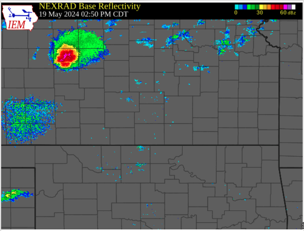
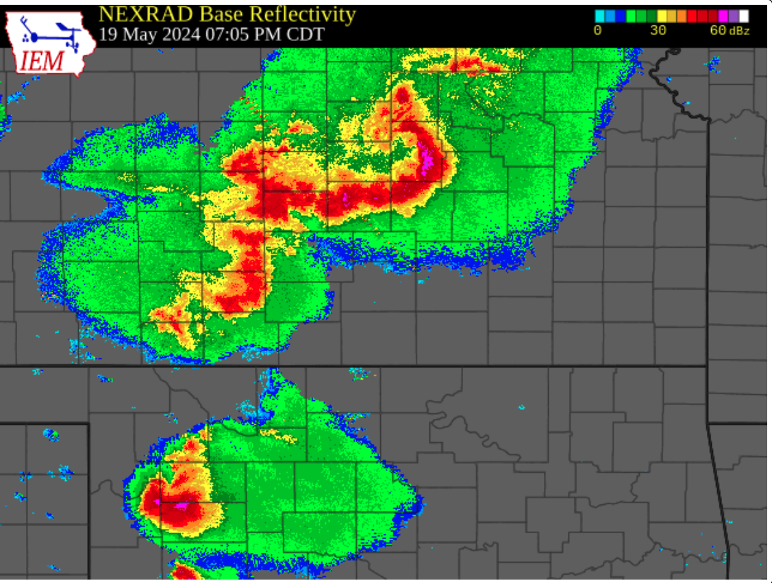
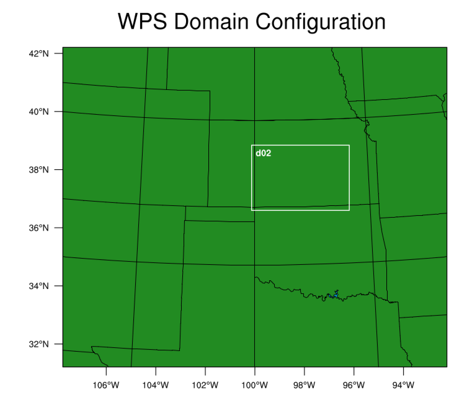
May 2024 Great Plains Severe Storm Event

This tutorial examines a Derecho and HP Supercell storm event that affected the Great Plains area on May 19th 2024. For more information on this event see weather.gov.

The figures below provides snapshots of the local radar during the evolution of the storm event. The left panel (05-19-2024 18:00 UTC) and middle panel (05-20-2024 00:00 UTC) illustrate the timing of storm development, whereas the right panel shows the nested domain configuration for WRF. The nested domain (d02) (0.1x0.1 degrees) is centered in Kansas, whereas the parent domain (d01) (0.2x0.2 degrees) covers a signifcant portion of the Great Plains.

The tutorial uses a 20 member ensemble initialized from the GFS at 05-19-2024 00:00 UTC. It performs an ensemble spinup from 00 to 06 UTC by applying perturbations to the GFS initial condition. It then assimilates atmospheric observations at 06 and 12 UTC respectively. Finally, a forecast is conducted (no observations assimilated) from 12 to 24 UTC. This sequence of ensemble spinup, assimilation mode and forecast mode generally follows published literature for atmospheric DA. Although we have strived to maintain scientific realism in this tutorial, we have made an effort to reduce the computational expense for reduced runtime by reducing the ensemble size (20) and coarsening the WRF spatial resolution (0.1 and 0.2 degrees). For science applications we recommend at least using 40 ensemble members which helps reduce sampling error and improves the assimlation performance.

On NSF NCAR’s Derecho,the tutorial requires roughly 40 minutes of computational run time, but can take longer depending upon the PBS queue wait time.

The goals of this tutorial are to: 1) provide an understanding of the major steps within a DA experiment, 2) port and test the WRF-DART scripts on the user’s system and 3) use the WRF-DART tutorial scripts as a template for the user’s own research application.

Important

The tutorial scripting and instructions are intended for the NSF NCAR supercomputer Derecho. The user must modify the scripts and interpret the instructions for other HPC systems. The scripting uses examples for a PBS (e.g. Derecho) and LSF queuing system. These will need to be modified for other systems (e.g. SLURM).

Step 1: Setup

There are several required dependencies for the executables and WRF-DART scripting components. On NSF NCAR’s Derecho, users have reported success building WRF, WPS, WRFDA, and DART using gfortan with the following module environment. Note: not all modules listed below are a requirement to compile and run the tutorial.

Currently Loaded Modules:
   1) ncarenv/23.09 (S)   3) udunits/2.2.28   5) ncarcompilers/1.0.0   7) cray-mpich/8.1.27   9) netcdf-mpi/4.9.2
   2) gcc/12.2.0          4) ncview/2.1.9     6) craype/2.7.23         8) hdf5-mpi/1.12.2    10) hdf/4.2.15

In addition, you’ll need to load the nco and ncl modules to run the set of scripts that accompany the tutorial. For Derecho the nco and ncl packages can be automatically loaded using the following commands:

module load nco
module load ncl/6.6.2

These commands are provided by default with the param.sh script. More details are provided below. There are multiple phases for the setup: building the DART executables, downloading the initial WRF boundary conditions, building (or using existing) WRF executables, and configuring and staging the scripting needed to perform an experiment.

Build the DART executables.

If you have not already, see Getting Started to download the DART software package. Set an environment variable DART_DIR to point to your base DART directory. How to do this will depend on which shell you are using.

shell	command
tcsh	setenv DART_DIR <path_to_your_dart_installation>
bash	export DART_DIR=<path_to_your_dart_installation>

In either case, you will replace <path_to_your_dart_installation> with the actual path to your DART installation. If you are using another shell, refer to your shell-specific documentation on how to set an environment variable.

Building the DART executables for the tutorial follows the same process as building any of the DART executables. Configure the mkmf.template file for your system, configure the input.nml for the model you want to compile, and run quickbuild.sh (which is not necessarily quick, but it is quicker than doing it by hand) to compile all the programs you might need for an experiment with that model.

1. It is assumed you have successfully configured the $DART_DIR/build_templates/mkmf.template file for your system. If not, you will need to do so now. See Getting Started for more detail, if necessary.

Important

If using gfortan to compile DART on Derecho, a successful configuration of the mkmf.template includes using the mkmf.template.gfortan script and customizing the compiler flags as follows: FFLAGS = -O2 -ffree-line-length-none -fallow-argument-mismatch -fallow-invalid-boz $(INCS)

2. [OPTIONAL] Modify the DART code to use 32bit reals. Most WRF/DART users run both the WRF model and the DART assimilation code using 32bit reals. This is not the default for the DART code. Make this single code change before building the DART executables to compile all reals as 32bit reals.

   Edit $DART_DIR/assimilation_code/modules/utilities/types_mod.f90 with your favorite editor. Change

   ! real precision:
   ! TO RUN WITH REDUCED PRECISION REALS (and use correspondingly less memory)
   ! comment OUT the r8 definition below and use the second one:
   integer, parameter :: r4 = SELECTED_REAL_KIND(6,30)
   integer, parameter :: r8 = SELECTED_REAL_KIND(12)   ! 8 byte reals
   !integer, parameter :: r8 = r4                      ! alias r8 to r4
   

   to

   ! real precision:
   ! TO RUN WITH REDUCED PRECISION REALS (and use correspondingly less memory)
   ! comment OUT the r8 definition below and use the second one:
   integer, parameter :: r4 = SELECTED_REAL_KIND(6,30)
   ! integer, parameter :: r8 = SELECTED_REAL_KIND(12)   ! 8 byte reals
   integer, parameter :: r8 = r4                      ! alias r8 to r4
   

3. Copy the tutorial DART namelist from $DART_DIR/models/wrf/tutorial/template_nest/input.nml.template to $DART_DIR/models/wrf/work/input.nml.

   cd $DART_DIR/models/wrf
   cp tutorial/template_nest/input.nml.template work/input.nml
   

4. Build the WRF-DART executables:

   cd $DART_DIR/models/wrf/work
   ./quickbuild.sh
   

   Many executables are built, the following executables are needed for the tutorial and will be copied to the right place by the setup.sh script in a subsequent step:

   advance_time
   fill_inflation_restart
   filter
   obs_diag
   obs_seq_to_netcdf
   obs_sequence_tool
   pert_wrf_bc
   wrf_dart_obs_preprocess
   

Preparing the experiment directory.

Create a “work” directory that can accomodate approximately 40 GB of space to run the tutorial. The rest of the instructions assume you have an environment variable called BASE_DIR that points to this directory. On Derecho it is convenient to use your scratch directory for this purpose.

shell	command
tcsh	setenv BASE_DIR <path_to_your_working_directory>
bash	export BASE_DIR=<path_to_your_working_directory>

1. The grib files required to generate WRF initial and boundary conditions and the observation files (obs_seq.out) have already been generated for you within a 10GB tar file. Put this file in your $BASE_DIR. Download the file directly to your local system:

   cd $BASE_DIR
   wget data.dart.ucar.edu/WRF/wrf_dart_nested_tutorial_15Jan2026.tar.gz
   tar -xzvf wrf_dart_nested_tutorial_15Jan2026.tar.gz
   

   After untarring the file you should see the following directories: icbc, output, perts, and template. The directory names (case sensitive) are important, as the scripts rely on these local paths and file names. Only the icbc and output folders contain files.

2. You will need template WRF namelists from the $DART_DIR/models/wrf/tutorial/template_nest directory:

   cp $DART_DIR/models/wrf/tutorial/template_nest/*.*   $BASE_DIR/template/.
   

3. You will also need scripting to run a WRF/DART experiment. Copy the contents of $DART_DIR/models/wrf/shell_scripts to the $BASE_DIR/scripts directory.

   mkdir $BASE_DIR/scripts
   cp -R $DART_DIR/models/wrf/shell_scripts/* $BASE_DIR/scripts
   

Note

There are also csh scripts available to run the nested tutorial example located here $DART_DIR/models/wrf/shell_scripts_csh/. We recommend the use of the bash scripting as shown in Step 3 as it has improved compatiblity with most HPC systems.

Build or locate the WRF, WPS and WRFDA executables

Instruction for donwloading the WRF package is located here. The WRF package consists of 3 parts: the WRF atmospheric model WRF(ARW), the WRF Preprocessing System (WPS) and WRF Data Assimilation System (WRFDA).

Importantly, DART is used to perform the ensemble DA for this tutorial, however, the WRFDA package is required to generate a set of perturbed initial ensemble member files and also to generate perturbed boundary condition files. The da_wrfvar.exe executable is required to generate a perturbation bank for the ensemble spinup step. Importantly, DART performs ensemble DA using the filter executable, whereas the WRFDA package is only used to generature perturbations. WRF_RUN directory for the tutorial.

WRF and WRFDA should be built with the “dmpar” option, while WPS can be built “serial”ly. See the WRF documentation for more information about building these packages.

Warning

For consistency and to avoid errors, you should build WRF, WPS, WRFDA, and DART with the same compiler you use for NetCDF. Likewise MPI should use the same compiler. You will need the location of the WRF and WRFDA builds to customize the param.sh script in the next step. If using gfortran to compile WRF on Derecho we recommend using option 34 (gnu dmpar) to configure WRF, option 1 (gnu serial) to configure WPS, and option 34 (gnu dmpar) to configure WRFDA. You will need the location of the WRF, WPS,and WRFDA builds to customize the param.sh script in the next step.

You should be compiling the traditional version of WRF designed for standard WRF forecasts and data assimilation workflows. These include executables such as real.exe, wrf.exe, and da_wrfvar.exe. You should not compile and use the wrfplus version of the model designed for variation assimilation algorithms (wrfplus.exe).

Using the gfortan compiler on Derecho required custom flag settings to successfully compile the WRF, WPS and WRFDA executables. For more information please see NCAR/DART github issue 627.

Configure $BASE_DIR/scripts/param.sh with proper paths and variables

The param.sh script sets variables which will be read by other WRF-DART scripts. There are some specific parameters for either the Derecho supercomputing system using the PBS queueing system or the (decommissioned) Yellowstone system which used the LSF queueing system. If you are not using Derecho, you may still want to use this script to set your queueing-system specific parameters.

Important

Make sure all the variables within param.sh as described in the table below are set appropriately. Remember, that Derecho HPC is used for the default settings.

Script variable	Description
module load nco	The nco package.
module load ncl/6.6.2	The ncl package.
BASE_DIR	The main working directory.
DART_DIR	The DART directory.
NUM_ENS	The total number of WRF ensemble members. The tutorial uses 20 for computational efficiency.
ASSIM_INT_HOURS	The frequency of assimilation steps, and temporal spacing between observations. This tutorial uses 6 hours.
ADAPTIVE_INFLATION	A DART tool used to adjust ensemble spread. We recommend to set to 1 (on) for assimilation mode in this example, however, users may opt to turn inflaton off for experiments where ensemble spread is large or model errors are small. The inflaton must be set to 0 (off) during forecast mode.
NUM_DOMAINS	The number of WRF domains. This tutorial uses a 2 domain setup (parent d01, nested d02). Scripting works for both single and multi-domains.
WRF_DM_SRC_DIR	The directory of the WRF dmpar installation.
WPS_SRC_DIR	The directory of the WPS installation.
VAR_SRC_DIR	The directory of the WRFDA installation.
GEO_FILES_DIR	The root directory of the WPS_GEOG files. NOTE: on Derecho these are available in the /glade/u/home/wrfhelp/WPS_GEOG directory
GRIB_DATA_DIR	The root directory of the GRIB data input into ungrib.exe. For this tutorial the grib files are included, so use ${ICBC_DIR}/grib_data
GRIB_SRC	The type of GRIB data (e.g. <Vtable.TYPE>) to use with ungrib.exe to copy the appropriate Vtable file. For the tutorial, the value should be ‘GFS’.
COMPUTER_CHARGE_ACCOUNT	The project account for supercomputing charges. See your supercomputing project administrator for more information.
EMAIL	An optional e-mail address used by the queueing system to send job summary information.

Now that param.sh is set properly, run the setup.sh script to create the proper directory structure and to move the executables and support files to the proper locations.

cd $BASE_DIR/scripts
./setup.sh param.sh

So far, your $BASE_DIR should contain the following directories:

icbc
obs_diag
obsproc
output
perts
post
rundir
scripts
template

Your $BASE_DIR/rundir directory should contain the following:

executables:

• advance_time,

• fill_inflation_restart,

• filter,

• obs_diag,

• obs_seq_to_netcdf,

• obs_sequence_tool,

• pert_wrf_bc (no helper page),

• wrf_dart_obs_preprocess

directories:

• WRFIN (empty)

• WRFOUT (empty)

• WRF_RUN (wrf executables and support files)

scripts:

• add_bank_perts.ncl

• new_advance_model.sh

support data:

• sampling_error_correction_table.nc

Check to make sure your $BASE_DIR/rundir/WRF_RUN directory contains:

da_wrfvar.exe
wrf.exe
real.exe
be.dat
contents of your WRF build run/ directory (support data files for WRF)

Note

Be aware that the setup.sh script is designed to remove $BASE_DIR/rundir/WRF_RUN/namelist.input. Subsequent scripting will modify $BASE_DIR/template/namlist.input.meso to create the namelist.input for the experiment.

For this tutorial, we are providing you with the namelist settings for a nested WRF domain which specifies the location, spatial resolution and relative positioning of the parent and nested domain. These namelist settings are used in conjunction with the grib files to generate the intial and boundary conditions.

Let’s now look inside the $BASE_DIR/scripts directory. You should find the following scripts:

Script name	Description
add_bank_perts.ncl	Applies perturbations to each WRF ensemble member to increase ensemble spread.
assim_advance.sh	Advances each WRF ensemble member between each assimilation time.
assimilate.sh	Runs filter at each assimilation time step.
diagnostics_obs.sh	Computes observation-space diagnostics and the model-space mean analysis increment.
driver.sh	Primary script for running the cycled analysis (DA) system.
first_advance.sh	Advances each WRF ensemble member during initial ensemble spinup.
gen_pert_bank.sh	Generates perturbations using WRFDA CV3.
gen_retro_icbc.sh	Generates the wrfinput and wrfbdy mean files for each assimilation time.
init_ensemble_var.sh	Performs the initial ensemble spinup.
mean_increment.ncl	Computes the mean state-space increment, which can be used for plotting.
new_advance_model.sh	Advances the WRF model in between assimilation times.
param.sh	Contains key variables and paths to run the WRF-DART system.
prep_ic.sh	Prepares the initial conditions for each WRF ensemble member.
real.sh	Runs the WRF real.exe program that advances WRF forward in time.
setup.sh	Creates the proper directory structure and puts executables/scripts in proper locations.

You will need to edit the following scripts in the table below to provide the paths to where you are running the experiment, to connect up files, and to set desired dates. Search for the string 'set this appropriately' for locations that you need to edit.

cd $BASE_DIR/scripts
grep -r 'set this appropriately' .

Other than param.sh, which was covered above, make the following changes:

File name	Variable / value	Change description
driver.sh	datefnl = 2024051912	Change to the final assimilation target date. In this example observations are assimilated at time steps 2024051906 and 2024051912.
gen_retro_icbc.sh	datea = 2024051900	Set to the starting time of the tutorial. This is the beginning time of the ensemble spinup, which runs for 6 hours until the first assimilation time step at 2024051906.
gen_retro_icbc.sh	datefnl = 2024052000	Set to the final time of the tutorial. This is the end of the forecast mode.
gen_retro_icbc.sh	paramfile = /full/path/to/param.sh	Script sources information from param.sh file.
gen_pert_bank.sh	datea = 2024051900	Set to the starting time of the tutorial.
gen_pert_bank.sh	num_ens = 60 (automatically set)	Total number of perturbation members. Automatically set to 3x model ensemble members (20).
gen_pert_bank.sh	paramfile = /full/path/to/param.sh	Script sources information from param.sh file.
gen_pert_bank.sh	savedir = ${PERTS_DIR}/work/boundary_perts.	Location of perturbation bank.
add_bank_pert.ncl	bank_size = 60 (automatically set)	Automatically set to 3x model ensemble members (20). If set manually it is recommended to set to the same value as gen_pert_bank.sh num_ens value. Cannot be greater than total perturbations in bank.

The setup is now complete. The tarred tutorial file provides the grib files and should be located within the $BASE_DIR/icbc directory that will be used to generate the WRF initial and boundary condition files. The $BASE_DIR/output directory contains the NCEP prepbufr observations (obs_seq.out) within each assimilation time sub-directory.

The $BASE_DIR/template directory should contain namelists for WRF, WPS, and DART.

Step 2: Create Initial and Boundary Conditions

We use GFS data to generate the initial and boundary conditions that will be used in the tutorial. The gen_retro_icbc.sh script executes a series of operations to extract the grib data, runs WPS executables geogrid, ungrib, metgrid, and then twice executes real.exe to generate a pair of WRF files and a boundary file for each analysis time and domain. These files are then added to a subdirectory corresponding to the date within the $BASE_DIR/output directory.

cd $BASE_DIR/scripts
./gen_retro_icbc.sh

Once the script completes, you should confirm the following files have been created within the $BASE_DIR/output/2024051900 directory:

wrfbdy_d01_154636_21600_mean
wrfinput_d01_154636_0_mean
wrfinput_d01_154636_21600_mean
wrfinput_d02_154636_0_mean
wrfinput_d02_154636_21600_mean

These filenames are appended with the Gregorian dates used within DART. Similar files (with different dates) should appear in all of the output sub-directories between the datea and datef dates set in the gen_retro_icbc.sh script.

Step 3: Generate Perturbation Bank

We use the WRFDA random CV option 3 to provide an initial set of random errors that we refer to as the ‘perturbation bank.’ During the subsequent ensemble spinup (Step 4) these perturbations are added to the deterministic, single instance GFS state generated in Step 2. Furthermore, during the subsequent assimilation cycling (Step 8), these perturbations are added to the forecast (target) boundary state, such that boundaries include random errors introducing uncertainty, which promotes ensemble spread to the WRF ensemble domain(s).

The spatial pattern and magnitude of the perturbations are controlled through the &wrfvar7 cv_options, as1, as2, as3 and as4 namelist settings included within the namelist.input.3dvar template. These settings were customized for this tutorial example. These will likely need to be modified for your own science application. For more information please see the WRFDA documentation.

cd $BASE_DIR/scripts
./gen_pert_bank.sh

The script will generate a batch job for each perturbation (60 total). The rule of thumb is to generate 3-4X as many perturbations as the model ensemble (20). This is done to increase the probability each ensemble member receives a unique perturbation. You should confirm the following files have been created within the $PERTS_DIR/work/boundary_perts directory:

pert_bank_mem_01.nc
pert_bank_mem_02.nc
..
..
pert_bank_mem_60.nc

Step 4: Perform Ensemble Spinup

Next, we generate an initial ensemble of WRF states to prepare for the first assimilation (analysis) step. We run the script init_ensemble_var.sh, which takes two arguments: a date string for the starting time and the path to the param.sh script.

The init_ensemble_var.sh script adds perturbations to the single instance WRF domain (generated in Step 2) which generates an ensemble of WRF simulations. Please note that the perturbations are chosen randomly and then added to the WRF state, thus the results of the tutorial should be qualitatively the same each time it is run, but because of the randomly chosen perturbations the DA results and diagnostics will not be deterministic. If there are multiple domains (like in this tutorial example) the code will automatically apply the perurbations from the parent domain to the nested domains through downscaling. This ensures that the location of perturbations are consistent across the domain boundaries. Next, the model ensemble is then advanced (spun-up) from the starting date (2024051900) to the first assimilation time (2024051906). To accomplish this, the init_ensemble_var.sh script orchestrates a series of calls as shown below:

1. add_bank_perts.ncl

2. first_advance.sh

3. new_advance_model.sh

This series of scripts executes wrf.exe to advance the WRF model using the following mpi run command within first_advance.sh as follows:

mpiexec -n 4 -ppn 4 ./wrf.exe

Please be aware that the mpi run command is customized for the Derecho environment. In addition, the processor setup was customized for the tutorial WRF domain setup. Please refer to the WRF documentation for more details on how to optimize the processor setup for other WRF domains. This script submits 20 batch jobs to the queuing system. It assumes a PBS batch system and the ‘qsub’ command for submitting jobs. If you have a different batch system, you will need to modify the commands such as #PBS and ‘qsub’. Fore more information you should familiarize yourself with running jobs on Derecho or your own HPC system.

The init_ensemble_var.sh script requires two command-line arguments - a date string for the starting time and the path to the param.sh script as shown below:

cd $BASE_DIR/scripts
./init_ensemble_var.sh 2024051900 param.sh

When the scripts complete for the all ensemble members, you should find 20 new files for each domain (40 total files) in the directory output/2024051900/PRIORS named prior_d01.0001, prior_d02.0001, etc.

Step 5: Prepare observations [Informational Only]

Important

The observation sequence (obs_seq.out) files used in this tutorial are already provided for you within the output directory. Proceed to step 7 if you wish to complete only the required tutorial steps. If you are interested in customizing a WRF-DART experiment for your own application, steps 5 and 6 provide useful guidance. The obs_seq.out files provided in this tutorial are generated from the NCEP PREPBUFR data files which are located at the NSF NCAR Geoscience Data Exchange (GDEX) (ds090 or ds337). Although we do not provide explicit instructions here to reconstruct the tutorial obs_seq.out files, you can follow the links for the prepbufr observation converter provided below. We used prepbufr data from the A26943-202405prepqmB.tar file that includes the date range for this tutorial (prepqm24051900.nr through prepqm24052100.nr).

Observation processing is critical to the success of running DART and is covered in Getting Started. In brief, to add your own observations to WRF-DART you will need to understand the relationship between observation definitions and observation sequences, observation types and observation quantities (see Step 6), and understand how observation converters extract observations from their native formats into the DART specific format.

Unlike many observation converters provided with DART, the PREPBUFR converter is unique because it requires the installation of an externally hosted package, and also involves a 2-stage conversion process (native format–>ascii–>obs_seq) as described below:

• Download PREPBUFR data from the NSF NCAR GDEX ds090 or ds337

• Unzip GDEX files, and locate the prepqm[YYMMDDHH].nr files of interest

• Install NCEP PREPBUFR text converter package (install.sh) See prepbufr

• Run PREPBUFR text conversion scripting (prepbufr.csh)

• Run text (ascii) to obs_seq executable (create_real_obs) See ascii_to_obs

Hint

The Quickstart Instructions included within the prepbufr link provided above is the fastest way to get started to convert your own PREPBUFR observations. The MADIS observation converter instructions are here.

Step 6: Overview of Forward Operators [Informational Only]

This section is for informational purposes only and does not include any required steps to complete the tutorial. It provides a description of the DART settings that control the forward operator which calculates the prior and posterior model estimates for the observations. An introduction to important namelist variables that control the operation of the forward operator are located in the WRF namelist documentation.

The obs_seq.out files provided with the tutorial contain over 10 different observation types (e.g. RADIOSONDE, AIRCRAFT etc). Here we examine a single temperature observation type. Please note that METAR type observations are not used in this tutorial example, but the file structure and concepts are exactly the same.

obs_sequence
obs_kind_definitions
          30
          41 METAR_TEMPERATURE_2_METER
..
..
  num_copies:            1  num_qc:            1
  num_obs:        70585  max_num_obs:        70585
NCEP BUFR observation
NCEP QC index
  first:            1  last:        70585
 OBS        1
   288.750000000000
   1.00000000000000
       -1       2          -1
obdef
loc3d
     4.819552185804497        0.6141813398083548         518.0000000000000     -1
kind
          41
 43200     152057
   3.06250000000000
..
..
..

A critical piece of observation metadata includes the observation type (METAR_TEMPERATURE_2_METER) which is linked to the quantity (QTY_2M_TEMPERATURE) through the observation definition file (obs_def_metar_mod.f90). This file is included within the &preprocess_nml section of the namelist file as:

&preprocess_nml
           overwrite_output = .true.
     input_obs_qty_mod_file = '../../../assimilation_code/modules/observations/DEFAULT_obs_kind_mod.F90'
    output_obs_qty_mod_file = '../../../assimilation_code/modules/observations/obs_kind_mod.f90'
     input_obs_def_mod_file = '../../../observations/forward_operators/DEFAULT_obs_def_mod.F90'
    output_obs_def_mod_file = '../../../observations/forward_operators/obs_def_mod.f90'
    quantity_files          = '../../../assimilation_code/modules/observations/atmosphere_quantities_mod.f90'
    obs_type_files          = '../../../observations/forward_operators/obs_def_reanalysis_bufr_mod.f90',
                             '../../../observations/forward_operators/obs_def_altimeter_mod.f90',
                             '../../../observations/forward_operators/obs_def_radar_mod.f90',
                             '../../../observations/forward_operators/obs_def_metar_mod.f90',
    ..
    ..
    ..

During the DART compilation described within Step 1 this information is included within the obs_def_mod.f90.

The vertical coordinate type is the 4th column beneath the loc3d header within obs_seq.out. In this example the value -1 indicates the vertical coordinate is VERTISSURFACE. It defines the vertical units of the observation (e.g. pressure, meters above sea level, model levels etc). This serves two purposes – foremost it is required during the vertical spatial interpolation to calculate the precise location of the expected observation. A second crtical function is that it defines whether it is a surface observation. Observations with a vertical coordinate of VERTISSURFACE are defined as surface observations. All other coordinates are considered non-surface observations (e.g. profile observations). Of note is that the vertical coordinate VERTISSURFACE and VERTISHEIGHT are functionally identical (i.e. meters above sea level), however only the VERTISSURFACE is a surface observation.

For more information on the vertical coordinate metadata see the detailed structure of an obs_seq file.

In order to connect this observation to the appropriate WRF output variables the wrf_state_variables within &model_nml defines the WRF field name and the WRF TYPE in the 1st and 3rd columns as shown in the tutorial example below:

&model_nml
  wrf_state_variables     = 'T2','QTY_TEMPERATURE','TYPE_T2','UPDATE','999'

..
..

For more information on the &model_nml variables see the WRF documentation page.

As described above, the linkage between the observation type and the WRF output field is defined through the physical quantity, surface variable designation (observation vertical coordinate), and WRF TYPE. The current design of the WRF model_mod.f90 is such that the quantity is a general classification (e.g. temperature, wind specific humidity), whereas the WRF TYPE classification is more precisely mapped to the WRF output field. The table below summarizes the dependency between the observation type and the WRF output field for a select number of observation types within the tutorial.

Note

The number of WRF output fields required to support an observation type can vary. For observation types where there is a direct analog to a WRF output field, the forward operator consists of only spatial interpolation, thus requires only a single output variable (e.g. METAR_TEMPERATURE_2_METER). For observation types that require multiple WRF output fields, the forward operator is more complex than a simple spatial interpolation. For more information see the notes below the table. A rule of thumb is a surface observation should use a surface output field (e.g. T2, U10). WRF surface output fields are appended by a numeric value indicating surface height in meters. It is possible to use a non-surface WRF output field (3D field) to estimate a surface observation, however, this requires a vertical interpolation of the 3D WRF field where the observed surface height does not coincide with the model levels. This either requires a vertical interpolation or an extrapolation which can be inaccurate and is not recommended.

DART Observation Type	Surface Obs ?	DART Quantity	WRF Type	WRF output field
METAR_TEMPERATURE_2_METER	Yes	QTY_2M_TEMPERATURE	TYPE_T2	T2
RADIOSONDE_TEMPERATURE	No	QTY_POTENTIAL_TEMPERATURE QTY_VAPOR_MIXING_RATIO QTY_PRESSURE QTY_GEOPOTENTIAL_HEIGHT	TYPE_T TYPE_QV TYPE_MU TYPE_GZ	THM QVAPOR MU PH
METAR_U_10_METER_WIND	Yes	QTY_U_WIND_COMPONENT QTY_V_WIND_COMPONENT	TYPE_U10 TYPE_V10	U10 V10
ACARS_U_WIND_COMPONENT	No	QTY_U_WIND_COMPONENT QTY_V_WIND_COMPONENT	TYPE_U TYPE_V	U V
METAR_DEWPOINT_2_METER	Yes	QTY_DEWPOINT QTY_SPECIFIC_HUMIDITY QTY_PRESSURE	TYPE_Q2 TYPE_PS	Q2 PSFC
RADIOSONDE_SPECIFIC_HUMIDITY	No	QTY_SPECIFIC_HUMIDITY	TYPE_QV	QVAPOR

Surface Temperature (e.g. METAR_TEMPERATURE_2_METER)

WRF output includes a direct analog for sensible temperature surface observations (e.g. T2), thus the forward operator requires only 1 variable to calculate the expected observation. The calculation includes a horizontal interpolation of the 2D temperature variable (e.g. T2).

Non-Surface Temperature (e.g. RADIOSONDE_TEMPERATURE)

In contrast to surface temperature observations, non-surface temperature observations require 4 WRF output fields. This is because observations are sensible temperature, whereas the 3D WRF temperature field is provided in perturbation potential temperature. Thus, the forward operator first requires a physical conversion between perturbation potential temperature to sensible temperature, followed by a spatial interpolation (this includes horizontal interpolation on WRF levels k and k+1, followed by vertical interpolation).

Important

There are two different 3D temperature WRF output fields that can work to calculate non- surface temperature observations (e.g. T or THM, T=THM when use_theta_m=0). However, and of utmost importance is the variable THM is required to be within the &model_nml if the 3D temperature field is to be updated in the filter step. This is because the WRF field *T* is a diagnostic variable with no impact on the forecast step, whereas the WRF field *THM* is a prognostic field which will impact the forecast.

Surface Wind (e.g. METAR_U_10_METER_WIND)

Surface winds have a direct WRF output analog (e.g. U10) and requires horizontal interpolation of the 2D zonal wind field. However, the meridional wind (e.g. V10) is also required in order to convert from modeled gridded winds to true wind observations. This requirement is an artifact of winds measured on a sphere being mapped on a 2D grid.

Non-Surface Wind (e.g. ACARS_U_WIND_COMPONENT)

This is identical to surface winds as described above, except the spatial interpolation requires horizontal interpolation on the k and k+1 WRF levels, followed by vertical interpolation.

Surface Dewpoint (e.g. METAR_DEWPOINT_2_METER)

The calculation of surface dewpoint requires a physical conversion using both surface pressure (PSFC) and surface vapor mixing ratio (Q2), follwed by horizontal interpolation.

Non-Surface Specific Humidity (e.g. RADIOSONDE_SPECIFIC_HUMIDITY)

Specific humidity observations require the (water) vapor mixing ratio (QVAPOR) for the forward operator. Although specific humidity and vapor mixing ratio are nearly identical, especially in dry air, they are actually two distinct physical properties – the ratio of water mass to total air mass versus ratio of water vapor mass to dry air mass respectively. Therefore the forward operator includes this physical conversion followed by a spatial interpolation (i.e. horizontal interpolation of k and k+1 WRF vertical levels followed by vertical interpolation).

Step 7: Create the First Set of Inflation Files

In this section we describe how to create the initial adaptive inflation files. These will be used by DART to control how the ensemble is inflated (increases spread) during the first assimilation cycle.

It is convenient to create initial inflation files before you start an experiment. The initial inflation files may be created with fill_inflation_restart, which was built by the quickbuild.sh step. A pair of inflation files is needed for each WRF domain.

Within the $BASE_DIR/rundir directory, the input.nml file has settings that control the behavior of fill_inflation_restart. Within this file there is the section:

&fill_inflation_restart_nml
   write_prior_inf = .true.
   prior_inf_mean  = 1.00
   prior_inf_sd    = 0.6

   write_post_inf  = .false.
   post_inf_mean   = 1.00
   post_inf_sd     = 0.6

   input_state_files = 'wrfinput_d01','wrfinput_d02'
   single_file       = .false.
   verbose           = .false.
   /

These settings create a prior inflation file with an inflation mean of 1.0 and a prior inflation standard deviation of 0.6. These are reasonable defaults to use. The input_state_files variable controls which file to use as a template. You can either modify this namelist value to point to one of the wrfinput_d01_XXX files under $BASE_DIR/output/<DATE>, for any given date, or you can copy one of the files to this directory. The actual contents of the file referenced by input_state_files do not matter, as this is only used as a template for the fill_inflation_restart program to write the default inflation values. Note that the number of files specified by input_state_files must match the number of domains specified in model_nml:num_domains, i.e. the program needs one template for each domain. This is a comma-separated list of strings in single ‘quotes’.

After running the program, the inflation files must then be moved to the directory expected by the driver.sh script.

Run the following commands with the dates for this particular tutorial:

cd $BASE_DIR/rundir
cp ../output/2024051900/wrfinput_d01_154636_0_mean ./wrfinput_d01
cp ../output/2024051900/wrfinput_d02_154636_0_mean ./wrfinput_d02
./fill_inflation_restart
mkdir ../output/2024051900/Inflation_input
mv input_priorinf_*.nc ../output/2024051900/Inflation_input/

Please note that the inflation files are manually generated and moved during the first assimilation time step only. During all subseqent times the inflation files are automatically generated and moved by the scripting.

Step 8: Perform the Assimilation (ASSIMILATION MODE)

We are now ready to assimilate observations. The driver.sh script accomplishes this through a series of scripts that 1) assimilates observations using the DART filter, 2) calculates observation space diagnostics for that assimilation time step, and 3) advances the WRF ensemble members to the next assimilation time step. It then repeats this cycle for the remaining assimilation steps. The sequence of scripts that are run are as follows:

1. prep_ic.sh (Extracts the DART state from the WRF prior state)

2. assimilate.sh (Executes DART filter and produces obs_seq.final)

3. diagnostic_obs.sh (Calculates observation space diagnostics: analysis_increment.nc, mean_increment.nc)

4. assim_advance.sh

5. new_advance_model.sh (Advances WRF model to next assimilation time)

6. add_bank_pert.ncl (Adds uncertainty to boundary conditions)

For each assimilation cycle there are two instances where a batch job is submitted to Derecho which uses an mpi run command. The first instance is during the execution of DART filter within assimilate.sh where filter is executed as follows:

mpiexec -n 256 -ppn 128 ./filter || exit 1

The second instance is during the advancement of the WRF ensemble to reach the next assimilation time step. This occurs within the assim_advance.sh script as follows:

mpiexec -n 4 -ppn 4 ./wrf.exe

Remember that (similar to Step 4) these batch sumbission commands are specific to the Derecho environment and the WRF domain. These will likely need to be modified to work for other WRF-DART science applications.

An important reminder is that driver.sh is the most complex step of the tutorial. A single forecast/assimilation cycle of this tutorial can take up to 10 minutes on Derecho - longer if debug options are enabled or if there is a wait time during the queue submission.

The main driver.sh script expects a starting date (YYYYMMDDHH) and the param.sh file as command line arguments. The run time output is redirected to a file named run.out. To assimilate the observations perform the following commands:

cd $BASE_DIR/scripts
./driver.sh 2024051906 param.sh >& run.out &

You can monitor the progress of the driver.sh execution by periodically viewing the run.out file. When the driver.sh is completed and successful the run.out file should print out: Reached the final date, Script exiting normally. In addition, a successful run will produce obs_seq.final, analysis_increment.nc and mean_incremant.nc files for each each assimilation time step located within ${OUTPUT_DIR}/2024051906, and ${OUTPUT_DIR}/2024051912.

If the script does not complete successfully based on the criteria just described, and viewing the run.out file provides inconclusive troubleshooting guidance, you must view the specific log files for the individual DART scripts located either in ${RUNDIR} or the ${RUNDIR}/advance_temp${ens} folders. These log files include: dart_log.out, assimilate_${datea}.0*, assim_advance_${ens}.o*, and add_perts.out. If there were problems during the WRF simulation you can view the WRF rsl.out.0000 and rsl.error.0000 files within ${RUNDIR}/advance_temp${ens}.

Important

During the execution of the driver.sh, immediately after the assimilation step, batch jobs are submitted to Derecho to advance the WRF model forward in time for each ensemble member. The script monitors the time from submission to successful completion. If the WRF job does not complete within the specified time (advance_thresh), then the script assumes that the job has failed and will resubmit 1 additional time before the script exits. The default behavior is that the advance_thresh is the same as the assigned walltime for the job (ADVANCE_TIME set in param.sh). This wait time is designed for this system setup (i.e. a responsive HPC like Derecho, and a tested WRF-DART setup). However, WRF jobs can exceed the advance_thresh if the job is queued for a long time, or if the WRF model fails. Long queue times can occur based on user demand and the priority of your job (ADVANCE_PRIORITY) set in param.sh. Furthermore it is not uncommon for the WRF model to fail for untested WRF-DART science applications where DART settings have not yet been optimized. In these cases you may have to adjust the advance_thresh or maximum retry setting.

Step 9: Perform the Forecast (FORECAST MODE)

The next step is to run the WRF model forecast to quantify the impact the assimilation of observations had on the forecast skill. This is a common step within the atmospheric DA literature. Here, we reuse the same driver.sh script as described in Step 8 except we modify the namelist settings to switch from assimilate to forecast mode.

First modify input.nml within ${RUN_DIR} such that the adaptive inflation is turned off by setting inf_flavor = 0. In addition, set all observation types to be evaluated as shown below:

&obs_kind_nml
    evaluate_these_obs_types = 'RADIOSONDE_TEMPERATURE',
                               'RADIOSONDE_U_WIND_COMPONENT',
                               'RADIOSONDE_V_WIND_COMPONENT',
                               'RADIOSONDE_SPECIFIC_HUMIDITY',
                               'RADIOSONDE_SURFACE_ALTIMETER',
                               'ACARS_U_WIND_COMPONENT',
                               'ACARS_V_WIND_COMPONENT',
                               'ACARS_TEMPERATURE',
                               'ACARS_DEWPOINT',
                               'SAT_U_WIND_COMPONENT',
                               'SAT_V_WIND_COMPONENT',
                               'GPSRO_REFRACTIVITY',
                               'PROFILER_U_WIND_COMPONENT',
                               'PROFILER_V_WIND_COMPONENT',
                               'METAR_U_10_METER_WIND',
                               'METAR_V_10_METER_WIND',
                               'METAR_TEMPERATURE_2_METER',
                               'METAR_DEWPOINT_2_METER',
                               'METAR_ALTIMETER',
                               'MARINE_SFC_U_WIND_COMPONENT',
                               'MARINE_SFC_V_WIND_COMPONENT',
                               'MARINE_SFC_TEMPERATURE',
                               'MARINE_SFC_ALTIMETER',
                               'MARINE_SFC_DEWPOINT',
                               'LAND_SFC_TEMPERATURE',
                               'LAND_SFC_U_WIND_COMPONENT',
                               'LAND_SFC_V_WIND_COMPONENT',
                               'LAND_SFC_ALTIMETER',
                               'LAND_SFC_DEWPOINT',
assimilate_these_obs_types  =  ''

Next, turn off the ensemble perturbation within add_bank_perts.ncl for both the ${RUNDIR} and ${BASE_DIR}/scripts as follows:

; Shuts off perturbations, only used for forecast mode
;perturbation scaling:
scale_T = 0.0
scale_U = 0.0
scale_V = 0.0
scale_Q = 0.0
scale_M = 0.0

Finally, turn off the adaptive inflation within the param.sh file by setting ADAPTIVE_INFLATION = 0.

Modify your driver.sh to run a forecast until 20240520 by setting datefnl = 2024052000. Then execute the following command:

cd ${BASE_DIR}/scripts
./driver.sh 2024051918 param.sh >& run.out &

To monitor the progress and success of the scripts follow the same guidance as described in Step 8. Remember all the steps and output files produced during forecast mode are nearly identical to assimilation mode. The only difference is that the scripting will not update the WRF state. We are performing an extended forecast (free) simulation.

Important

The purpose of the forecast mode is to be run only after all assimilation steps are completed, thus providing a assessment of forecast skill performance that is common for atmospheric DA science publications. Once forecast mode has been completed the user should not switch back to assimilation mode because the inflation files will not be available. Forecast mode should not be used in an attempt to skip certain assimilation time steps with reduced or no observations. Instead, the inflation setting should be modified to account for observations that strongly vary in space and time. See the inflation documentation for more details.

Step 10: Diagnose the Assimilation and Forecast Results

Once you have successfully completed steps 1-9, it is important to check the quality of the assimilation. In order to do this, DART provides analysis system diagnostics in both state and observation space. Here we provide instructions to diagnose performance based on a single assimilation time step (2024051912). However, be aware that you can perform these same diagnostics for any assimilation/forecast performed during the tutorial. We leave that as an exercise to be performed on your own.

Important

If the tutorial is performed successfully your diagnostic plots should look similar to the figures shown here, but they will not be identical because the assimilation results are not deterministic. This is primarily because the perturbations are randomly chosen to generate the ensemble spread. This influences all subsequent steps in the tutorial and will lead to unique results.

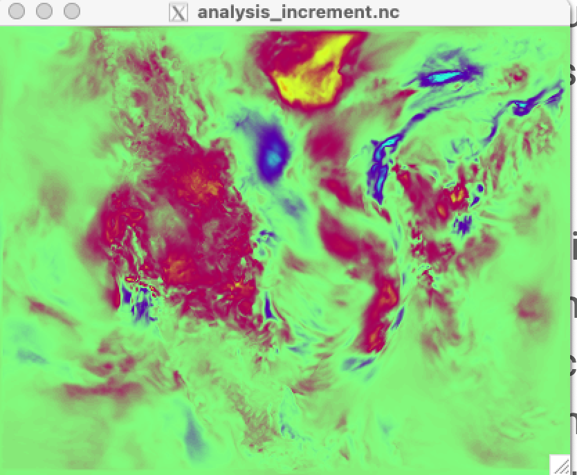
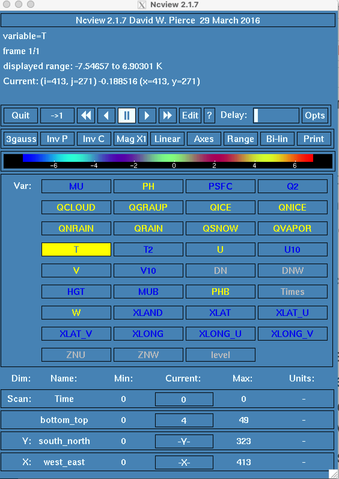
As a preliminary check, confirm that the analysis system actually updated the WRF state. Locate the file in the $BASE_DIR/output/2024051912 directory called analysis_increment_d01.nc which is the difference of the ensemble mean state between the background (prior) and the analysis (posterior) after running filter. Use a tool, such as ncview, to look at this file as follows:

cd $BASE_DIR/output/2024051912
module load ncview
ncview analysis_increment_d01.nc

The analysis_increment_d01.nc file includes the following atmospheric variables: such as MU, PH, PSFC, QRAIN, QCLOUD, QGRAUP, QICE, QNICE, QSNOW, QVAPOR, THM, U, V and T2. The example figure below shows the increments for QVAPOR (water vapor mixing ratio) only. You can use ncview to advance through all atmospheric pressure levels, by clicking on the “bottom_top” button within the ncview gui. You should see spatial patterns that look something like the meteorology of the day.

For more information on how the increments were calculated, we recommend that you review the Diagnostics Section of the DART Documentation. There are seven sections within the diagnostics section including 1) Checking your initial assimilation, 2) Computing filter increments and so on. Be sure to advance through all the sections.

The existence of increments proves the model state was adjusted, however, this says nothing about the quality of the assimilation. For example, how many of the observations were assimilated? Does the posterior state better represent the observed conditions of the atmosphere? These questions can be addressed with the tools described in the remainder of this section. All of the diagnostic files (obs_epoch.nc and obs_diag_output.nc) have already been generated from the tutorial. (driver.sh executes diagnostics_obs.sh). Therefore you are ready to start the next sections.

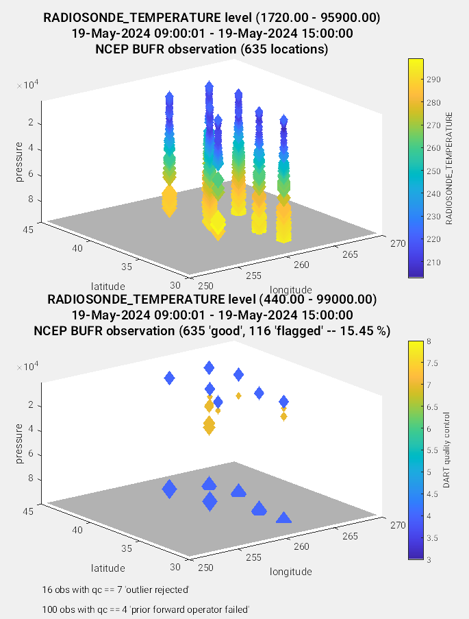
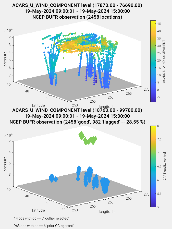
Visualize the observation locations and acceptance rate

The example below uses the plot_obs_netcdf.m script to visualize the observation type: RADIOSONDE_TEMPERATURE which includes both horizontal and vertical coverage across North America. We recommend to view the script’s contents with a text editor, paying special attention to the beginning of the file which is notated with a variety of examples. Then to run the example do the following:

cd $DARTROOT/diagnostics/matlab
module load matlab
matlab -nodesktop

Within Matlab declare the following variables, then run the script plot_obs_netcdf.m as follows below being sure to modify the fname variable for your specific case.

>> fname = '$BASEDIR/output/2024051912/obs_epoch_002.nc';
>> ObsTypeString = 'RADIOSONDE_TEMPERATURE'; % 'ACARS_U_WIND_COMPONENT'
>> region        = [250 270 30 45 -Inf Inf];
>> CopyString    = 'NCEP BUFR observation';
>> QCString      = 'DART quality control';
>> maxgoodQC     = 2;
>> verbose       = 1;   % anything > 0 == 'true'
>> twoup         = 1;   % anything > 0 == 'true'
>> plotdat = plot_obs_netcdf(fname, ObsTypeString, region, CopyString, QCString, maxgoodQC, verbose, twoup);

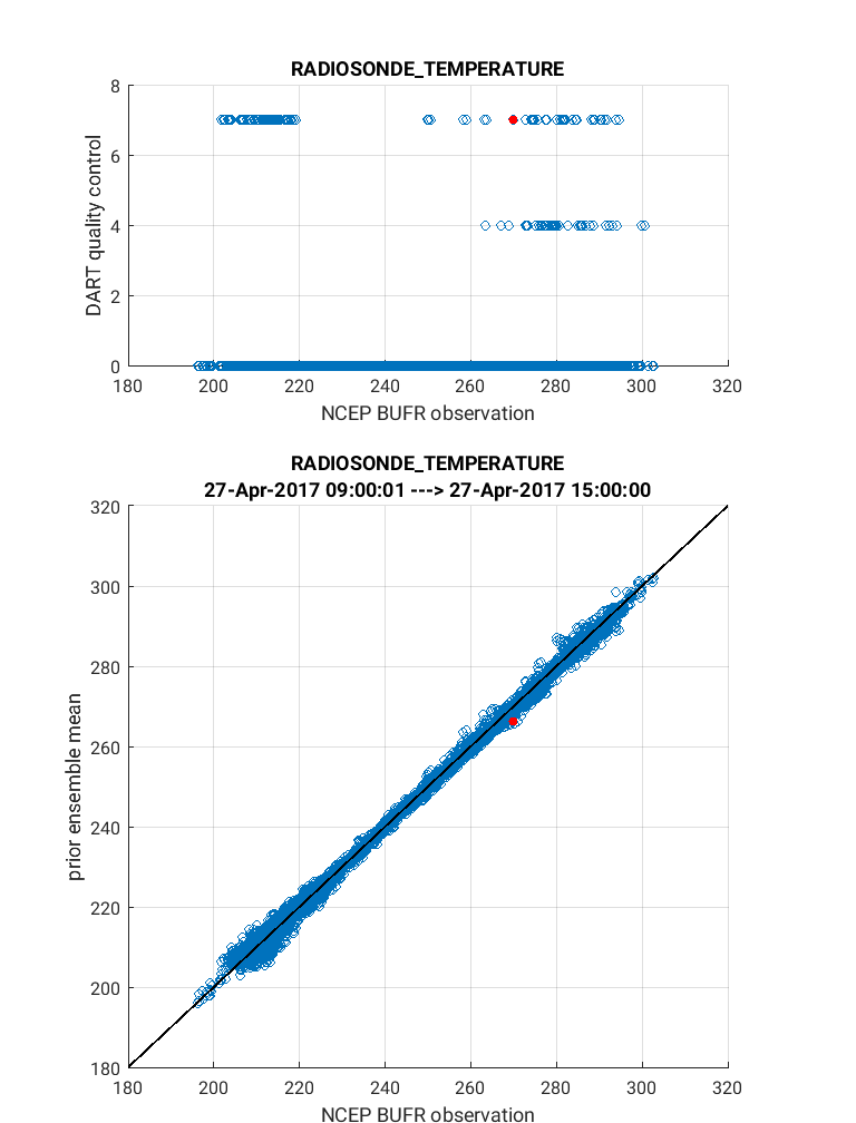
Below are two examples of the figure produced by plot_obs_netcdf.m for observations of RADIOSONDE_TEMPERATURE (left) and ACARS_U_WIND_COMPONENT (right) respectively. Note that the top panel includes both the 3-D location of all possible observations, which are color-coded based upon the temperature or wind value. The bottom panel, on the other hand, provides only the location of the observations that were rejected by the assimilation. The color code indicates the reason for the rejection based on the DART quality control (QC). In this example observations were rejected based on violation of the outlier threshold (QC = 7), and forward operator failure (QC = 4). Text is included within the figures that give more details regarding the rejected observations (bottom left of figure), and percentage of observations that were rejected (flagged, located within title of figure).

Tip

The user can manually adjust the appearance of the data by accessing the ‘Rotate 3D’ option either by clicking on the top of the figure or through the menu bar as Tools > Rotate 3D. Use your cursor to rotate the map to the desired orientation.

The plot_obs_netcdf.m also provides information for all the observations available for assimilation at that time step. You can adjust the ObsTypeString setting to examine one observation type at a time.

N =   1019      RADIOSONDE_U_WIND_COMPONENT (type   1) tween levels 470.00 and 99000.00
N =   1019      RADIOSONDE_V_WIND_COMPONENT (type   2) tween levels 470.00 and 99000.00
N =    751           RADIOSONDE_TEMPERATURE (type   5) tween levels 440.00 and 99000.00
N =    312     RADIOSONDE_SPECIFIC_HUMIDITY (type   6) tween levels 30000.00 and 99000.00
N =      1        AIRCRAFT_U_WIND_COMPONENT (type  12) tween levels 21660.00 and 21660.00
N =      1        AIRCRAFT_V_WIND_COMPONENT (type  13) tween levels 21660.00 and 21660.00
N =   3440           ACARS_U_WIND_COMPONENT (type  16) tween levels 17870.00 and 99780.00
N =   3440           ACARS_V_WIND_COMPONENT (type  17) tween levels 17870.00 and 99780.00
N =   3375                ACARS_TEMPERATURE (type  18) tween levels 17870.00 and 99780.00
N =      7     RADIOSONDE_SURFACE_ALTIMETER (type  40) tween levels 195.00 and 1095.00
N =     25               LAND_SFC_ALTIMETER (type  43) tween levels 141.00 and 2299.00

Next we will demonstrate the use of the link_obs.m script which provides visual tools to explore how the observations impacted the assimilation. The script generates 3 different figures which includes a unique linking feature that allows the user to identify the features of a specific observation including physical location, QC value, and prior/posterior estimated values. In the example below the ‘linked’ observation appears ‘red’ in all figures. To execute link_obs.m do the following within Matlab being sure to modify fname for your case:

>> clear all
>> close all
>> fname = '$BASEDIR/output/2024051912/obs_epoch_002.nc';
>> ObsTypeString = 'RADIOSONDE_TEMPERATURE';
>> region        = [250 270 30 45 -Inf Inf];
>> ObsCopyString = 'NCEP BUFR observation';
>> CopyString    =  'prior ensemble mean';
>> QCString      = 'DART quality control';
>> global obsmat;
>> link_obs(fname, ObsTypeString, ObsCopyString, CopyString, QCString, region)

Tip

To access the linking feature, click near the top of the figure such that a list of icons appear. Next click on the ‘brush data’ icon then click on a data point you wish to link. It will appear red. Alternatively you can access the brush tool through the menu bar (Tools > Brush).

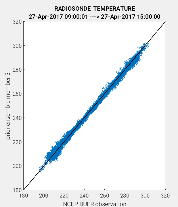
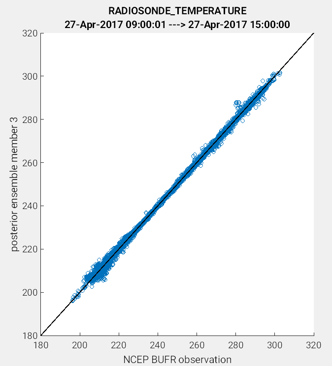
Another useful application of the link_obs.m script is to visualize the improvement of the model estimate of the observation through the 1:1 plot. One way to do this is to compare the prior and posterior model estimate of either the ensemble mean or a single ensemble member. In the example figures below, a 1:1 plot was generated for the prior and posterior values for ensemble member 3. (Left Figure: CopyString =  'prior ensemble member 3' and Right Figure: CopyString = posterior ensemble member 3'). Note how the prior member estimate (left figure) compares less favorably to the observations as compared to the posterior member estimate (right figure). The improved alignment (blue circles closer to 1:1 line) between the posterior estimate and the observations indicates that the DART filter update provided an improved representation of the observed atmospheric state.

So far the example figures have provided primarily qualitative estimates of the assimilation performance. The next step demonstrates how to apply more quantitative measures to assess assimilation skill.

Quantification of model-observation mismatch and ensemble spread

The plot_rmse_xxx_profile.nc script is one of the best tools to evaluate assimilation performance across a 3-D domain such as the atmosphere. It uses the obs_diag_output.nc file as an input to generate RMSE, observation acceptance and other statistics. Here we choose the ensemble ‘total spread’ statistic to plot alongside RMSE, however, you can choose other statistics including ‘bias’, ‘ens_mean’ and ‘spread’. For a full list of statistics perform the command ncdump -v CopyMetaData obs_diag_output.nc. The figure below illustrates vertical profile statistics for observations of RADIOSONDE_TEMPERAURE (left) and ACARS_U_WIND_COMPONENT (right).

>> fname ='$BASEDIR/output/2024051912/obs_diag_output.nc';
>> copy = 'totalspread';
>> obsname = 'RADIOSONDE_TEMPERATURE';  %ACARS_U_WIND_COMPONENT
>> plotdat = plot_rmse_xxx_profile(fname,copy,'obsname',obsname)

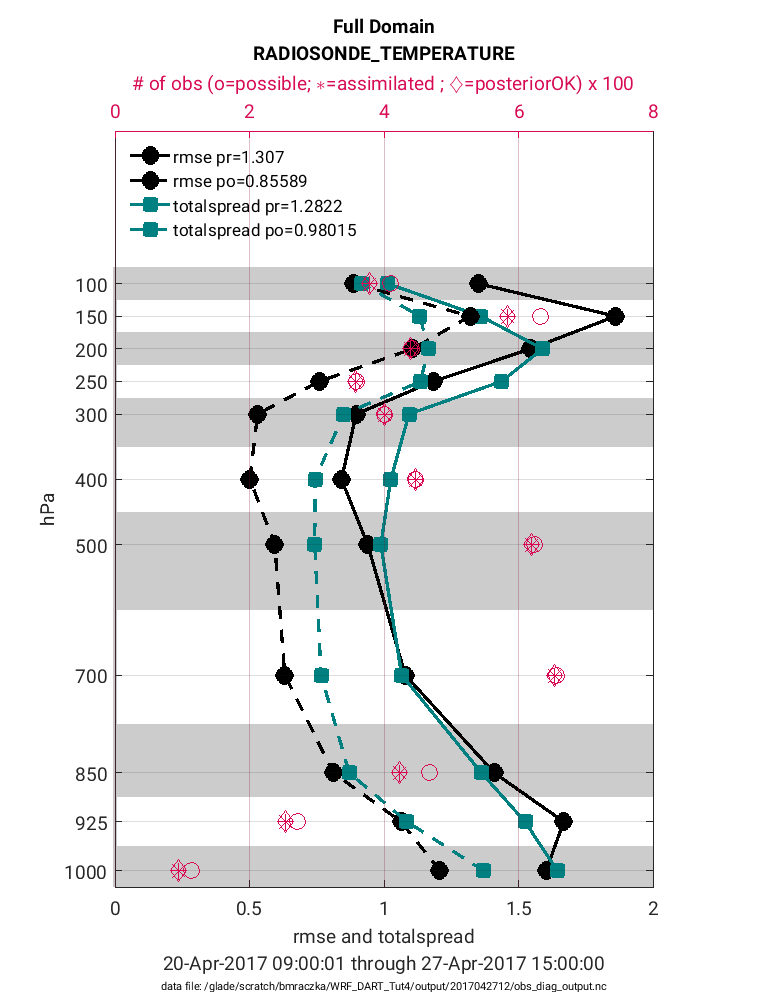
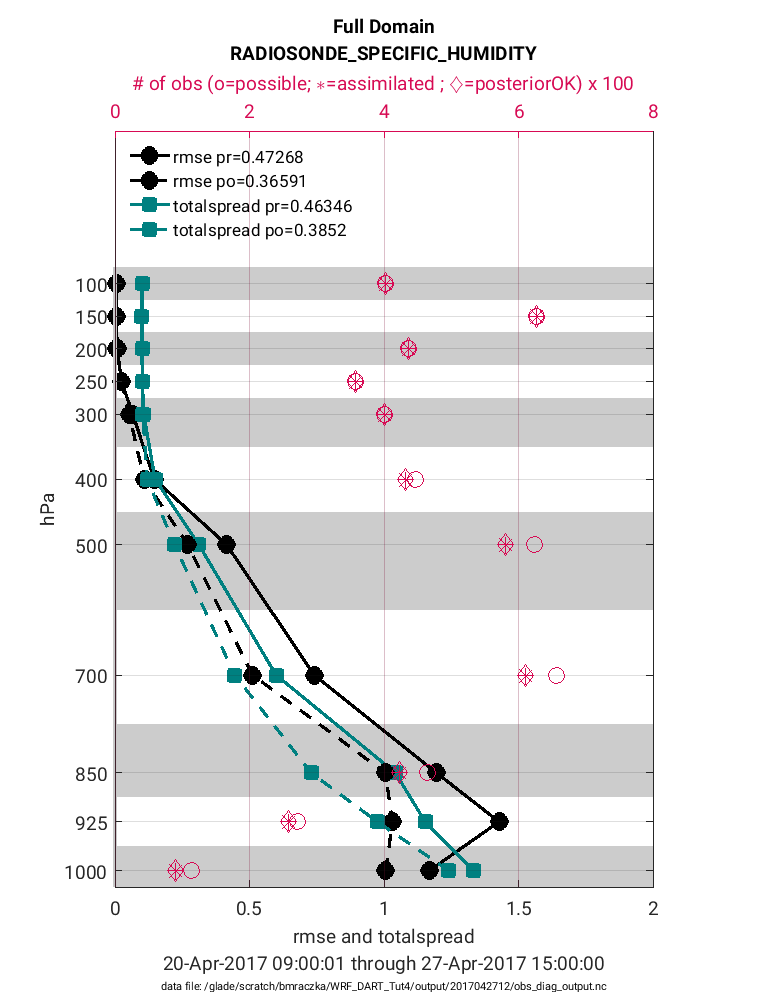
Note in the figure above that the prior RMSE and total spread values (solid black and teal lines) are significantly greater than the posterior values (dashed black and teal lines). This is exactly the behavior we would expect (desire) because the decreased RMSE indicates the posterior model state has an improved representation of the atmosphere. It is common for the introduction of observations to also reduce the ‘total spread’ because the prior ensemble spread will compress to better match the observations. In general, it is preferable for the magnitude of the total spread to be similar to the RMSE. If there are strong departures between the total spread and RMSE this suggests the adaptive inflation settings may need to be adjusted to avoid filter divergence. Note that these statistics are given for each pressure level (1-11) within the WRF model. Accompanying each level is also the total possible (pink circle) and total assimilated (pink asterisk) observations. Note that for each level the percentage of assimilated observations is quite high (>90%). This high acceptance percentage is typical of a high-quality assimilation and consistent with the strong reduction in RMSE.

Remember, a full list of observations rejection criteria are provided here. Regardless of the reason for the failure, a successful simulation assimilates the vast majority of observations as shown in the figure above.

Although the plot_rmse_xxx_profile.m script is valuable for visualizing vertical profiles of assimilation statistics, it doesn’t capture the temporal evolution. Temporal evolving statistics are valuable because the skill of an assimilation often begins poorly because of biases between the model and observations, which should improve with time. Also the quality of the assimilation may change because of changes in the quality of the observations. In these cases the plot_rmse_xxx_evolution.m script is used to illustrate temporal changes in assimilation skill.

This time evolving diagnostic works best when all the assimilation times steps are combined into one obs_diag.output.nc file, however the obs_diag_output.nc files automatically generated during the tutorial are for indivdual assimilation times. We leave it as an exercise on your own to generate a custom obs_diag_output.nc that combines several different assimilation time steps. Please use the instructions in the next section as a guide.

Generating the obs_diag_output.nc and obs_epoch*.nc files manually [OPTIONAL]

This step is optional because the WRF-DART Tutorial automatically generates the diagnostic files (obs_diag_output.nc and obs_epoch_*.nc). However, these files were generated with pre-set options (e.g. spatial and temporal domains, and bin size etc.) that you may wish to modify. Therefore this section describes the steps to generate the diagnostic files directly from the DART scripts by using the WRF Tutorial as an example.

Generating the obs_epoch*.nc file

cd $DARTROOT/models/wrf/work

Generate a list of all the obs_seq.final files for all steps in the tutorial. This command creates a text list file.

ls ${BASE_DIR}/output/2024*/obs_seq.final > obs_seq_tutorial.txt

The DART exectuable obs_seq_to_netcdf is used to generate the obs_epoch type files. Modify the obs_seq_to_netcdf and ‘schedule’ namelist settings (using a text editor like vi) with the input.nml file to specify the spatial domain and temporal binning. The values below are intended to include the entire time period of the assimilation.

&obs_seq_to_netcdf_nml
  obs_sequence_name = ''
  obs_sequence_list = 'obs_seq_tutorial.txt',
  lonlim1 =   0.0
  lonlim2 = 360.0
  latlim1 = -90.0
  latlim2 =  90.0
  verbose = .false.
  /

&schedule_nml
  calendar       = 'Gregorian',
  first_bin_start =  1601, 1, 1, 0, 0, 0,
  first_bin_end   =  2999, 1, 1, 0, 0, 0,
  last_bin_end   =   2999, 1, 1, 0, 0, 0,
  bin_interval_days    = 1000000,
  bin_interval_seconds = 0,
  max_num_bins         = 1000,
  print_table          = .true
  /

Finally, run the exectuable:

./obs_seq_to_netcdf

This should generate obs_epoch*.nc files.

Generating the obs_diag_output.nc file

cd $DARTROOT/models/wrf/work

The DART exectuable obs_diag is used to generate the obs_diag_output files. Modify the obs_diag namelist settings (using a text editor like vi) with the input.nml file to specify the spatial domain and temporal binning. Follow the same steps to generate the obs_seq_tutorial.txt file as described in the previous section.

&obs_diag_nml
  obs_sequence_name = '',
  obs_sequence_list = 'obs_seq_tutorial.txt',
  first_bin_center =  2024, 5, 19, 0, 0, 0 ,
  last_bin_center  =  2024, 5, 19, 18, 0, 0 ,
  bin_separation   =     0, 0, 0, 6, 0, 0 ,
  bin_width        =     0, 0, 0, 6, 0, 0 ,
  time_to_skip     =     0, 0, 0, 0, 0, 0 ,
  max_num_bins  = 1000,
  Nregions   = 1,
  lonlim1    =   0.0,
  lonlim2    = 360.0,
  latlim1    = 10.0,
  latlim2    = 65.0,
  reg_names  = 'Full Domain',
  print_mismatched_locs = .false.,
  verbose = .true.
  /

Finally, run the exectuable:

./obs_diag

This should produce an obs_diag_output.nc file.

If you encounter difficulties setting up, running, or evaluating your system performance, please consider contact DART support at dart(at)ucar(dot)edu.

Additional materials from previous in-person tutorials

• Introduction - DART Lab materials

• WRF-DART basic building blocks -slides (some material is outdated)

• Computing environment support -slides

• WRF-DART application examples -slides (some material is outdated)

• Observation processing -slides

• DART diagnostics - observation diagnostics

More Resources

• Check or Submit DART Issues

• DAReS website

• Preparing MATLAB to use with DART.

• WRF model users page