CLM5-DART Tutorial
Introduction
This tutorial describes how to set up a simple assimilation using CLM5-DART. The expectation is that the user is very familiar with running CLM off-line and thus the tutorial focuses upon the specific aspects of integrating CLM with DART. Once completed, the goal is that the user should be familar enough with the concepts of CLM5-DART in order to design an assimilation for their own research interests.
This tutorial was assembled to be compatible with CLM5.0.34 as part
of CESM (release-cesm2.2.01) or CTSM (release-cesm2.2.03) and the latest release on the main branch of the
the DART repository.
Other combinations of CLM and DART (prior to DART version 9.13.0) may not be compatible
with this tutorial. Currently, only the CTSM (release-cesm2.2.03) is fully compatible with Derecho.
If you are using other tags you may need to modify the external scripting to be compatible
with Derecho.
It is not recommended to use this tutorial without prior experience with running and understanding CLM. If new to CLM we recommend you attend a CLM tutorial or review the CLM documentation including the Technical Description, User Guide, and use the CESM User Forum for CLM-specific assistance.
If you are new to DART, we recommend that you become familiar by first working through the DART Tutorial and then understanding the DART getting started documentation.
This CLM5-DART tutorial is based on a simple example in which we describe how to:
set up the software
review concepts of assimilation
provide a specific example of how CLM and DART interact in an assimilation framework
If you wish to move beyond this tutorial and address a unique/new research question be prepared to invest a significant amount of time to modify the CLM-DART setup. In general, a CLM-DART simulation that is running without errors, does not mean it has been optimized for performance. Optimal performance requires the evaluation of assimilation diagnostics (e.g. observation acceptance rate, RMSE and bias between modeled and observed properties) and making additional modifications to the setup scripts. Examples of setup modifications include changes to localization, inflation, observations that are assimilated, updated model state variables, assimilation time window, assimilation frequency, and the model and observation grid resolution.
We encourage users to complete the tutorial and then modify CLM-DART to pursue their own research questions. We have comprehensive and searchable documentation, with trained and experienced staff that can help troubleshoot issues (dart@ucar.edu).
Tutorial Overview
The tutorial is a simplified global simulation that assimilates daily observations for up to a maximum of 10 days. A total of 5 observations are distributed across the globe that includes observations of leaf area, biomass, snow cover, and soil temperature. The observations are ‘synthetic’ meaning they have been generated from the output of a separate CLM simulation with random error added. Synthetic observations are generally easier to assimilate than real-world observations because they remove systemic differences between the model and observations. This assimilation uses a 5-member ensemble (i.e. 5 CLM simulations run simultaneously). An ensemble is required within Ensemble Kalman Filter (EnKF) data assimilation to calculate the modeled covariance amongst the state variables in CLM. The covariance amongst the CLM state variables dictates how the CLM model state is updated during the assimilation step given a set of observations. The beginning of the assimilation starts from near present day (January-2011) and is initalized in ‘hybrid’ mode from a set of CLM restart files generated from a previous CLM 5-member ensemble simulation. The atmospheric forcing used for the assimilation comes from the Community Atmospheric Model (CAM) reanalyses (CAM6 and CAM4). This reanalysis atmospheric data includes 80 total ensemble members in which the across-member variation represents atmospheric uncertainty. We use 5 different ensemble members from the CAM6 reanalysis to generate spread within this CLM5-DART tutorial simulation.
Note
This CLM5-DART tutorial has been simplified to reduce run-time and computational expense. For research applications an assimilation is typically run for many model months/years. In addition a 5-member ensemble is generally too small to properly sample model uncertainty and we recommend 80, but no less than 40 ensemble members for research applications.
The goal of this tutorial is to demonstrate how CLM5 and DART interact to perform data assimilation to provide an observation-constrained simulation of CLM. This requires setting numerous namelist/input values that control the configuration of CLM and DART setup.
After running this tutorial, you should be able to understand the major steps involved in setting up your own data assimilation experiments. However, you will need to do additional work to customize the CLM5-DART system for your particular research needs. For example, this tutorial provides both the initial conditions and observation sequence files to simplify the process and are specific to the tutorial, whereas you will need to generate custom initial conditions and observation sequence files for your own work.
Important
We have provided tutorial instructions for the NSF NCAR supercomputer Derecho, however, if using your own machine you will need to customize the setup scripts in order to properly compile DART (see Step 4: Compiling DART). These system-specific setup steps may take a good deal of effort, especially if you are unfamiliar with details such as compilers, MPI, NetCDF libraries, batch submission systems etc. To perform this tutorial we assume the user is comfortable with LINUX operating systems as well as using text editors (e.g. vi, nedit, emacs) to edit the CLM5-DART setup scripts and namelist files etc.
Other required files to run the tutorial include the meteorology (Step 5), reference case (Step 6), and observation files (Step 7). These are all readily available if you are using Derecho. If you are using your own machine you need use the following links to download these files directly:
CAM6 Reanalysis Meteorology `CAM6, Year 2011, ensemble members 1-5 for three separate file types:
f.e21.FHIST_BGC.f09_025.CAM6assim.011.cpl_000{1-5}.ha2x3h.2011.ncf.e21.FHIST_BGC.f09_025.CAM6assim.011.cpl_000{1-5}.ha2x1hi.2011.ncf.e21.FHIST_BGC.f09_025.CAM6assim.011.cpl_000{1-5}.ha2x1h.2011.ncReference Case and Observations,
clm5_dart_tutorial_2022_03_01.tar.gz
Step 1: Download CLM5
CLM is continually being updated by the model developer and user community
consisting of both NSF NCAR and university scientists and researchers.
In contrast, DART is maintained by a relatively small group that supports
numerous earth system models (20+) including CLM. Therefore the DART team
focuses on only supporting official released versions of CLM. This documentation
and scripting was tested using the CESM tag release-cesm2.2.0 and
release-cesm2.2.03 following
the download instructions here.
Although the DART code may work with more recent versions of CESM (CLM) we recommend
checking out release-cesm2.2.03 which is compatible with both DART and Derecho
git clone https://github.com/ESCOMP/CTSM.git cesm_dart
cd cesm_dart
git checkout release-cesm2.2.03
./manage_externals/checkout_externals
Adding CLM5 SourceMods
Some minor modifications have to be made to the CLM5 source code in order to be run with DART. Most importantly, these include skipping several balance checks in CLM5 for the time step immediately after the assimilation update step. These sourcecode modifications are brought in through the SourceMod mechanism in CLM where modifications overwrite the template sourcecode during the compilation step. The SourceMods are included within the DART package which is downloaded in Step 2.
For more information on the SourceMods see the main CLM-DART documentation.
Compiling CLM5
Compiling CLM5 on the NSF NCAR machine Derecho is straightforward because the
run and build environment settings are already defined within the config_machines.xml
file located within the CESM installation: <cesmroot>/cime/config/cesm/machines. If
you are using your own machine please follow the porting instructions located
here.
When performing a CLM5-DART assimilation run, the compiling step for CLM5 occurs within
the CLM5_setup_assimilation script described later within this tutorial.
Step 2: Download DART
The tutorial material is available within the most recent release of the DART repository on the main branch.
cd /glade/work/$USER/
git clone https://github.com/NCAR/DART.git
cd DART
Step 4: Compiling DART
Similar to CLM, it is necessary to compile the DART code before an assimilation
can be performed. The DART code includes a variety of build template scripts that provide
the appropriate compiler and library settings depending upon your system environment.
This is an example of the system environment for Derecho (e.g. module list),
which was used to perform this tutorial:
Currently Loaded Modules:
  1) ncarenv/23.06 (S)   2) intel/19.0.5   3) ncarcompilers/1.0.0   4) hdf5/1.12.2   5) netcdf/4.9.2
Please note in this example we used the intel fortran compiler with netcdf libraries
to support the netcdf file format and the mpt libraries to support the mpi tasks.
Below are instructions on how to modify the DART template script mkmf_template
to properly compile DART on Derecho:
cd DART/build_templates
cp mkmf.template.intel.linux mkmf.template
Confirm the mkmf_template has the following settings:
MPIFC = mpif90
MPILD = mpif90
FC = ifort
LD = ifort
...
...
INCS = -I$(NETCDF)/include
LIBS = -L$(NETCDF)/lib -lnetcdff -lnetcdf
FFLAGS  = -O -assume buffered_io $(INCS)
LDFLAGS = $(FFLAGS) $(LIBS)
Next we will test to make sure the DART scripts can be run correctly,
by compiling and executing the preprocess script. The preprocess
script must be run before the core DART code is compiled because
it writes the source code that supports the observations.
This provides the necessary support for the specific
observations that we wish to assimilate into CLM. For more information
see the preprocess documentation.
First make sure the list of obs_def and obs_quantity module source codes
are contained in the &preprocess_nml namelist within the input.nml.
cd DART/models/clm/work
vi input.nml
Note
We use the vi editor within the tutorial instructions, but we recommend that you use the text editor you are most comfortable with. To close the vi editor follow these instructions from stackoverflow.
This example uses namelist setting that specifically loads obs_def and
obs_quantity commonly used for land DA, including models like CLM.
Confirm the &preprocess_nml settings are as follows:
&preprocess_nml
   input_obs_qty_mod_file  = '../../../assimilation_code/modules/observations/DEFAULT_obs_kind_mod.F90'
   output_obs_qty_mod_file = '../../../assimilation_code/modules/observations/obs_kind_mod.f90'
   input_obs_def_mod_file  = '../../../observations/forward_operators/DEFAULT_obs_def_mod.F90'
   output_obs_def_mod_file = '../../../observations/forward_operators/obs_def_mod.f90'
   obs_type_files          = '../../../observations/forward_operators/obs_def_land_mod.f90',
                             '../../../observations/forward_operators/obs_def_tower_mod.f90',
                             '../../../observations/forward_operators/obs_def_COSMOS_mod.f90'
   quantity_files          = '../../../assimilation_code/modules/observations/land_quantities_mod.f90',
                             '../../../assimilation_code/modules/observations/space_quantities_mod.f90'
                             '../../../assimilation_code/modules/observations/atmosphere_quantities_mod.f90'
   /
Next run quickbuild.sh to build and run preprocess and build the dart exectuables:
./quickbuild.sh
Confirm the new source code has been generated for
DART/observations/forward_operators/obs_def_mod.f90
and DART/assimilation_code/modules/observations/obs_kind_mod.f90
Step 5: Setting up the atmospheric forcing
A requirement for Ensemble Kalman Filter (EnKF) type DA approaches is to generate multiple model simulations (i.e. a model ensemble) that quantifies 1) state variable uncertainty and 2) correlation between state variables. Given the sensitivity of CLM to atmospheric conditions an established method to generate multi-instance CLM simulations is through weather reanalysis data generated from a CAM-DART assimilation. These CAM-DART reanalyses are available from 1997-2010 CAM4, and 2011-2020 CAM6.
For this tutorial we will use the January 2011 CAM6 reanalysis (d345000) only.
To make sure the scripts can locate the weather data first make sure
the DART_params.csh variable dartroot is set to the path of your
DART installation. For example, if you have a Derecho account and you
followed the DART cloning instructions in Step 2 above your dartroot
variable will be: /<your Derecho work directory>/DART. Make sure you update
the default dartroot as shown below.
setenv dartroot /glade/work/${USER}/DART
Next confirm within the CLM5_setup_assimilation script that the path (${SOURCEDIR}/${STREAMFILE_*})
to all four of your atmospheric stream file templates (e.g. datm.streams.txt.CPLHISTForcing.Solar*)
is correct. In particular make sure the SOURCEDIR variable is set correctly below:
set STREAMFILE_SOLAR        = datm.streams.txt.CPLHISTForcing.Solar_single_year
set STREAMFILE_STATE1HR     = datm.streams.txt.CPLHISTForcing.State1hr_single_year
set STREAMFILE_STATE3HR     = datm.streams.txt.CPLHISTForcing.State3hr_single_year
set STREAMFILE_NONSOLARFLUX = datm.streams.txt.CPLHISTForcing.nonSolarFlux_single_year
...
...
# Create stream files for each ensemble member
set SOURCEDIR = ${dartroot}/models/clm/shell_scripts/cesm2_2
${COPY} ${SOURCEDIR}/${STREAMFILE_SOLAR}         user_${FILE1} || exit 5
${COPY} ${SOURCEDIR}/${STREAMFILE_STATE1HR}      user_${FILE2} || exit 5
${COPY} ${SOURCEDIR}/${STREAMFILE_STATE3HR}      user_${FILE3} || exit 5
${COPY} ${SOURCEDIR}/${STREAMFILE_NONSOLARFLUX}  user_${FILE4} || exit 5
Next, edit each of your atmospheric stream file templates to make sure the
filePath within domainInfo and fieldInfo below is set correctly to
reference the CAM6 reanalysis file. The example below is for
datm.streams.txt.CPLHISTForcing.nonSolarFlux_single_year. Repeat this for
all four of the template stream files including for Solar, State1hr
and State3hr.
<domainInfo>
     <variableNames>
        time          time
        doma_lon      lon
        doma_lat      lat
        doma_area     area
        doma_mask     mask
     </variableNames>
     <filePath>
        /glade/campaign/collections/rda/data/d345000/cpl_unzipped/NINST
     </filePath>
     <fileNames>
        f.e21.FHIST_BGC.f09_025.CAM6assim.011.cpl_NINST.ha2x3h.RUNYEAR.nc
     </fileNames>
  </domainInfo>
  ...
  ...
  ...
  <fieldInfo>
     <variableNames>
        a2x3h_Faxa_rainc     rainc
        a2x3h_Faxa_rainl     rainl
        a2x3h_Faxa_snowc     snowc
        a2x3h_Faxa_snowl     snowl
        a2x3h_Faxa_lwdn      lwdn
     </variableNames>
     <filePath>
          /glade/campaign/collections/rda/data/d345000/cpl_unzipped/NINST
     </filePath>
     <offset>
        1800
     </offset>
     <fileNames>
        f.e21.FHIST_BGC.f09_025.CAM6assim.011.cpl_NINST.ha2x3h.RUNYEAR.nc
     </fileNames>
  </fieldInfo>
Selected variables within atmospheric stream file
Description
filePath
Directory of CAM6 reanalysis file. For tutorial, this only includes year 2011, with ensemble members 1-5. During execution of
CLM5_setup_assimilationthe textNINSTis replaced with ensemble member number0001-0005. The ensemble member number is set through thenum_instancesvariable located inDART_params.csh.fileNames
The CAM6 reanalysis file name. For the tutorial, this only includes year 2011, with ensemble members 1-5. The
NINSTvariable is replaced in the same way as described above forfilepath. For this tutorial theRUNYEARvariable will be replaced by2011. TheRUNYEARvariable is set throughstream_year_firstlocated withinDART_params.csh.variableNames
Meteorology variables within CAM6 reanalysis. First column is variable name within netCDF reanalysis file, whereas the second column is the meteorology variable name recognized by CLM.
Finally, edit the DART_params.csh file such that the RUNYEAR and NINST variables
within the atmospheric stream templates are replaced with the appropriate year and
ensemble member. To do this confirm the settings within DART_params.csh are as follows:
setenv num_instances  5

 ..
 ..

setenv stream_year_align 2011
setenv stream_year_first 2011
setenv stream_year_last  2011
Step 6: Setting up the initial conditions for land earth system properties
The initial conditions for the assimilation run are prescribed (all state variables
from the top of vegetation canopy to subsurface bedrock) by a previous 5-member ensemble
run (Case: clm5.0.06_f09_80) that used the same CAM6 reanalysis to generate initial spread
between ensemble members. This is sometimes referred to as an ensemble ‘spinup’. This
ensemble spinup was run for 10 years to generate sufficient spread amongst ensemble members
for this tutorial.
Note
The proper ensemble spinup time depends upon the specific research application. In general, the goal is to allow the differences in meterological forcing to induce changes within the CLM variables that you plan to adjust during the DART update step. CLM variables that have relatively quick response to atmospheric forcing (e.g. leaf area, shallow-depth soil variables) require less spinup time. However, other CLM variables take longer to equilibrate to atmospheric forcing (e.g. biomass, soil carbon).
This initial ensemble spinup was run with resolution f09_09_mg17 (0.9x1.25 grid resolution)
with compset 2000_DATM%GSWP3v1_CLM50%BGC-CROP_SICE_SOCN_MOSART_SGLC_SWAV (CESM run with
only land and river components active). The starting point of the assimilation is run in
CLM ‘hybrid’ mode which allows the starting date of the assimilaton to be different than
the reference case, and loosens the requirements of the system state. The tradeoff is that
restarting in hybrid mode does not provide bit-by-bit reproducible simulations.
For the tutorial, set the DART_parms.csh variables such that the end of the
ensemble spinup (at time 1-1-2011) are used as the initial conditions for the assimilation:
setenv refcase      clm5.0.06_f09_80
setenv refyear      2011
setenv refmon       01
setenv refday       01
setenv reftod       00000
...
...
setenv stagedir /glade/campaign/cisl/dares/glade-p-dares-Oct2023/RDA_strawman/CESM_ensembles/CLM/CLM5BGC-Crop/ctsm_${reftimestamp}
...
...
setenv start_year    2011
setenv start_month   01
setenv start_day     01
setenv start_tod     00000
Important variables to set initial conditions |
Description |
|---|---|
refcase |
The reference casename from the spinup ensemble that serves as the starting conditions for the assimilation. |
refyear, refmon, refday reftod |
The year, month, day and time of day of the reference case that the assimilation will start from. |
stagedir |
The directory location of the reference case files. |
Step 7: Setting up the observations to be assimilated
In ‘Step 4: Compiling DART’ we have already completed an important
step by executing preprocess which generates source code
(obs_def_mod.f90, obs_kind_mod.f90) that supports the assimilation of observations
used for this tutorial. In this step, we compile these observation definitions in to the DART
executables. The observations are read into the
assimilation through an observation sequence file whose format is described
here.
First confirm that the baseobsdir variable within DART_params.csh
is pointed to the directory where the observation sequence files are
located. In Derecho they are located in the directory as:
setenv baseobsdir /glade/campaign/cisl/dares/glade-p-dares-Oct2023/Observations/land
In this tutorial we have several observation types that are to be
assimilated, including SOIL_TEMPERATURE, MODIS_SNOWCOVER_FRAC,
MODIS_LEAF_AREA_INDEX and BIOMASS. To enable the assimilation
of these observations types they must be included within
the &obs_kind_nml within the input.nml file as:
&obs_kind_nml
  assimilate_these_obs_types = 'SOIL_TEMPERATURE',
                               'MODIS_SNOWCOVER_FRAC',
                               'MODIS_LEAF_AREA_INDEX',
                               'BIOMASS',
  evaluate_these_obs_types   = 'null'
  /
Below is an example of a single observation (leaf area index)
within an observation sequence file used within this tutorial (obs_seq.2011-01-02-00000):
OBS            3
6.00864688253571
5.44649167346675
0.000000000000000E+000

obdef
loc3d
   5.235987755982989         0.000000000000000        -888888.0000000000     -2
kind
        23
   0     149750
0.200000000000000
Below is the same portion of the file as above, but with the variable names:
<Observation sequence number>
<Observation Value>
<True Observation Value>
<Observation Quality Control>

obdef
loc3d
   <longitude>    <latitude>     <vertical level>     <vertical code>
kind
  <observation quantity number>
     <seconds>    <days>
<Observation error variance>
Observation Sequence File Variable |
Description |
|---|---|
observation sequence number |
The chronological order of the observation within the observation sequence file. This determines the order in which the observation is assimilated by DART for a given time step. |
observation value |
The actual observation value that the DART |
true observation value |
The observation generated from CLM output. In this case the observation was generated as part of a perfect model experiment (OSSE; Observing System Simulation Experiment), thus the ‘true’ value is known. |
observation quality control |
The quality control value provided from the data provider. This can be used as a filter in which to exclude low quality observations from the assimilation. |
longitude, latitude |
Horizontal spatial location of the observation in radians |
level, vertical level type code |
Vertical observation location in units defined by vertical level type |
observation type number |
The DART observation type assigned to the obervation type
(e.g. |
second, days |
Time of the observations in reference to Jan 1, 1601 |
observation error variance |
Uncertainty of the observation Value |
Now that we have set both the path to the observation sequence files, and the types of observations
to be assimilated, confirm the quality control settings within the &quality_control_nml of
the input.nml file are as follows:
&quality_control_nml
   input_qc_threshold = 1.0
   outlier_threshold  = 3.0
   /
Quality Control Namelist |
Description |
|---|---|
input_qc_threshold |
The quality control value that is provided from the observation product. Any value above this threshold will cause the observation to be rejected and ignored during the assimilation step. |
outlier threshold |
The observation is rejected if: (prior mean - observation) > (expected difference x outlier threshold). The prior mean is is calculated from the CLM model ensemble mean, and the expected difference is the square root of the sum of the square uncertainty of the prior mean and observation uncertainty. |
These quality control settings do not play a role in this tutorial because we are using synthetic observations which are, by design, very close to the model output. Thus, in this tutorial example, systematic biases between the model and observations are removed. However, in the case of real observations, it is common for large systemic differences to occur between the model and observations either because 1) structural/parametric error exists within the model or 2) model or observation uncertainty is underestimated. In these cases it is beneficial to reject observations to promote a stable simulation and prevent the model from entering into unrealistic state space.
Note
This tutorial already provides properly formatted synthetic observations for the user, however, when using ‘real’ observations for research applications DART provides observation converters. Observation converters are scripts that convert the various data product formats into the observation sequence file format required by the DART code. Observations converters most relevant for land DA and the CLM model include those for leaf area, flux data, snow, and soil moisture here and here. Even if an observation converter is not available for a particular data product, it is generally straightforward to modify them for your specific application.
Step 8: Setting up the DART and CLM states
Defining the DART state space is a critical part of the assimilation setup process. This serves
two purposes, first, it defines which model variables are used in the forward operator. The forward operator
is defined as any operation that converts from model space to observation space to create the
‘expected observation’. The mismatch between the true and expected observation forms the foundation
of the model update in the DART filter step.
In this tutorial, observations of SOIL_TEMPERATURE, MODIS_SNOWCOVER_FRAC,
MODIS_LEAF_AREA_INDEX, and BIOMASS are supported by specific clm variables. See the table
below which defines the dependency of each DART observation type upon specific DART quantities
required for the forward operator. We also include the CLM variables that serve as the DART
quantities for this tutorial:
DART Observation Type |
DART Observation Quantities |
CLM variables |
|---|---|---|
|
|
|
|
|
|
|
|
|
|
|
|
Note
For this tutorial example most of the observation types rely on a single quantity
(and CLM variable) to calculate the expected observation. For these the CLM
variable is spatially interpolated to best match the location of the observation.
The BIOMASS observation type is an exception in which 3 quantities are required
to calculate the expected observation. In that case the sum of the CLM
variables of leaf, live stem and structural (dead) carbon represents the biomass observation.
Second, the DART state space also defines which portion of the CLM model state is updated by DART.
In DA terminology, limiting the influence of the observations to a subset of the CLM model
state is known as ‘localization’ which is discussed more fully in Step 9.
In theory the complete CLM model state may be updated based on the relationship with the observations.
In practice, a smaller subset of model state variables, that have a close physical relationship with
the observations, are included in the DART state space. In this tutorial, for example, we limit
the update to CLM variables most closely related to biomass, leaf area, soil temperature and
snow. Modify the &model_nml within input.nml as below:
&model_nml
  ...
  ...
  clm_variables  = 'leafc',       'QTY_LEAF_CARBON',            '0.0', 'NA', 'restart' , 'UPDATE',
                   'frac_sno',    'QTY_SNOWCOVER_FRAC',         '0.0', '1.', 'restart' , 'NO_COPY_BACK',
                   'SNOW_DEPTH',  'QTY_SNOW_THICKNESS',         '0.0', 'NA', 'restart' , 'NO_COPY_BACK',
                   'H2OSOI_LIQ',  'QTY_SOIL_LIQUID_WATER',      '0.0', 'NA', 'restart' , 'UPDATE',
                   'H2OSOI_ICE',  'QTY_SOIL_ICE',               '0.0', 'NA', 'restart' , 'UPDATE',
                   'T_SOISNO',    'QTY_TEMPERATURE',            '0.0', 'NA', 'restart' , 'UPDATE',
                   'livestemc',   'QTY_LIVE_STEM_CARBON',       '0.0', 'NA', 'restart' , 'UPDATE',
                   'deadstemc',   'QTY_DEAD_STEM_CARBON',       '0.0', 'NA', 'restart' , 'UPDATE',
                   'TLAI',        'QTY_LEAF_AREA_INDEX',        '0.0', 'NA', 'vector'  , 'NO_COPY_BACK',
                   'TSOI',        'QTY_SOIL_TEMPERATURE',       'NA' , 'NA', 'history' , 'NO_COPY_BACK'
  /
The table below provides a description for each of the columns for clm_variables within
&model_nml.
Column |
Description |
|---|---|
1 |
The CLM variable name as it appears in the CLM netCDF file. |
2 |
The corresponding DART QUANTITY. |
3 |
Minimum value of the posterior.
If set to ‘NA’ there is no minimum value.
The DART diagnostic files will not reflect this value, but
the file used to restart CLM will.
|
4 |
Maximum value of the posterior.
If set to ‘NA’ there is no maximum value.
The DART diagnostic files will not reflect this value, but
the file used to restart CLM will.
|
5 |
Specifies which file should be used to obtain the variable.
'restart' => clm_restart_filename'history' => clm_history_filename'vector' => clm_vector_history_filename |
6 |
Should
filter update the variable in the specified file.'UPDATE' => the variable is updated.'NO_COPY_BACK' => the variable remains unchanged. |
There are important distinctions about the clm_variables as described above.
First, any clm variable whether it is a restart, history or vector file can be used
as a forward operator to calculate the expected observation. Also if the 6th column
is defined as UPDATE, then that variable is updated during the filter step
regardless of the CLM variable type. However, in order for the update step to have a
permanent effect upon the evolution of the CLM model state, the update must be applied to a
prognostic variable in CLM – which is always the restart file. Updates to restart
file variables alters the file thus changing the initial conditions for the next time
step. The CLM history and vector files, on the other hand, are diagnostic variables
with no impact on the evolution of the model state.
A second important distinction amongst clm_variables is that the restart file
state variables are automatically generated after each CLM simulation time step, thus are readily
available to include within the DART state. In contrast, the history or vector file variables
must be manually generated through the user_nl_clm file within CLM. This is generated
within the portion of the CLM5_setup_assimilation script as shown below. Modify this
portion of the CLM5_setup_assimilation script so that it appears as follows:
...
...
echo "hist_empty_htapes = .true."                                      >> ${fname}
echo "hist_fincl1 = 'NEP','H2OSOI','TSOI','EFLX_LH_TOT','TLAI'"        >> ${fname}
echo "hist_fincl2 = 'NEP','FSH','EFLX_LH_TOT_R','GPP'"                 >> ${fname}
echo "hist_fincl3 = 'NEE','H2OSNO','TLAI','TWS','SOILC_vr','LEAFN'"    >> ${fname}
echo "hist_nhtfrq = -$stop_n,1,-$stop_n"                               >> ${fname}
echo "hist_mfilt  = 1,$h1nsteps,1"                                     >> ${fname}
echo "hist_avgflag_pertape = 'A','A','I'"                              >> ${fname}
echo "hist_dov2xy = .true.,.true.,.false."                             >> ${fname}
echo "hist_type1d_pertape = ' ',' ',' '"                               >> ${fname}
The hist_fincl setting generates history files (fincl1->h0; fincl2->h1;
fincl3->h2) for each of the clm variables as defined above. The
hist_dov2xy setting determines whether the history file is output
in structured gridded format (.true.) or in unstructured, vector history format (.false.).
Most of the history files variables in this example are provided just for illustration, however,
the tutorial requires that the TLAI variable is output in vector history format.
The restart, history and vector files define domains 1, 2 and 3 respectively
within DART. The restart domain (domain 1) must always be defined, however domains 2 and 3 are optional.
In this tutorial example all 3 domains are required, where domain 2 corresponds to the
h0 history file, and domain 3 corresponds with the h2 history files.
Step 9: Set the spatial localization
Localization is the term used to restrict the portion of the state to regions
related to the observation. Step 8 is a type of localization in that it restricts
the state update to a subset of CLM variables. Here, we further restrict the influence
of the observation to the state space most nearly physically collocated with the observation.
The spatial localization is set through the the assim_tools_nml, cov_cutoff_nml
and location_nml settings within input.nml as:
# cutoff of 0.03 (radians) is about 200km
&assim_tools_nml
   cutoff                          = 0.05
&cov_cutoff_nml
  select_localization = 1
  /
&location_nml
   horiz_dist_only             = .true.
Localization namelist variable |
Description |
|---|---|
|
Value (radians) of the half-width of the localization radius.
At 2* |
|
Defines a function that determines the decreasing impact an observation has on the model state. Value of 1 is the Gaspari-Cohn function. |
|
If |
In some research applications (not this tutorial) it may also be important to
localize in the vertical direction. For land modeling this could be important
for soil carbon or soil moisture variables which typically only have observations
near the land surface, whereas the model state is distributed in layers well
below the surface. For vertical localization the horiz_dist_only must be set
to .false. For more information on localization see
assim_tools_mod.
Step 10: Set the Inflation
Generating and maintaining ensemble spread during the assimilation allows for the covariance to be calculated between model state variables (that we want to adjust) and the expected observation. The strength of the covariance determines the model update. For CLM-DART assimilations the ensemble spread is generated through a boundary condition: the atmospheric forcing as described in Step 5. However, because the number of ensemble members is limited and boundary condition uncertainty is only one source of model uncertainty, the true ensemble spread is undersampled. To help compensate for this we employ inflation during the assimilation which changes the spread of the ensemble without changing the ensemble mean. The inflation algorithm computes the ensemble mean and standard deviation for each variable in the state vector in turn, and then moves the member’s values away from the mean in such a way that the mean remains unchanged.
Although inflation was originally designed to account for ensemble sampling errors, it has also been demonstrated to help address systemic errors between models and observations as well. More information on inflation can be found here.
In this tutorial we implement a time and space varying inflation (inflation flavor 5: enhanced spatial-varying; inverse gamma) such that the inflation becomes an added state property which is updated during each assimilation step similar to CLM state variables. The inflation state properties include both a mean and standard deviation. The mean value determines how much spread is added across the ensemble (spread is generated when mean > 1). The standard deviation defines the certainty of the mean inflation value, thus a small value indicates high certainty and slow evolution of the mean with time. Conversely a high standard deviation indicates low certainty and faster evolution of the inflation mean with time.
Modify the inflation settings within input.nml for the &filter_nml and
the &fill_inflation_restart_nml as follows:
Note
The &filter_nml has two columns, where column 1 is for prior inflation
and column 2 is for posterior inflation. We only use prior inflation for
this tutorial, thus inf_flavor=0 (no inflation) for column 2.
&filter_nml

  ...
  ...
  ...
  inf_flavor                  = 5,                       0
  inf_initial_from_restart    = .true.,                 .false.
  inf_sd_initial_from_restart = .true.,                 .false.
  inf_deterministic           = .true.,                  .true.
  inf_initial                 = 1.0,                     1.0
  inf_lower_bound             = 0.0,                     1.0
  inf_upper_bound             = 20.0,                   20.0
  inf_damping                 = 0.9,                     0.9
  inf_sd_initial              = 0.6,                     0.6
  inf_sd_lower_bound          = 0.6,                     0.6
  inf_sd_max_change           = 1.05,                    1.05
&fill_inflation_restart_nml
   write_prior_inf   = .true.
   prior_inf_mean    = 1.00
   prior_inf_sd      = 0.6
   ...
   ...
Inflation namelist variable |
Description |
|---|---|
|
The inflation algorithm type as described below:
|
|
If |
|
If |
|
If |
|
Initial value of inflation if not read from restart file |
|
Lower bound of inflation mean value |
|
Upper bound of inflation mean value |
|
Damping factor for inflation mean values. The difference
between the current inflation value and 1.0 is multiplied by
this factor and added to 1.0 to provide the next inflation
mean. An |
|
Initial value of inflation standard deviation if not read from restart file. If ≤ 0, do not update the inflation values, so they are time-constant. If positive, the inflation values will adapt through time. |
|
Lower bound for inflation standard deviation. If using a negative value for inf_sd_initial this should also be negative to preserve the setting. |
|
For |
|
Setting this to |
|
Initial value of prior inflation mean when
|
|
Initial value of prior inflation standard deviation when
|
It is also important to confirm that the domains defined in Step 8 (restart, history, vector)
are the same as what is defined in the &fill_inflation_restart_nml and &filter_nml namelist settings.
Confirm the input and output file list account for all 3 domains as:
&filter_nml
   input_state_file_list    = 'restart_files.txt',
                              'history_files.txt',
                              'vector_files.txt'
   output_state_file_list   = 'restart_files.txt',
                              'history_files.txt',
                              'vector_files.txt'
&fill_inflation_restart_nml
  input_state_files = 'clm_restart.nc','clm_history.nc','clm_vector_history.nc'
  single_file       = .false.
Important
The input_state_file_list, output_state_file_list and input_state_files must match the domains
that were defined in Step 8.
The assimilate.csh script assigns the CLM file that defines each domain. In this tutorial
the restart, history and vector domains are defined by the .r.,
.h0. and .h2. files respectively. *We show the portions of the assimilate.csh script
below for illustration purposes only. Do not modify these lines for the tutorial.*
The domains are set within the Block 4: DART INFLATION portion of the
script as:
set     LND_RESTART_FILENAME = ${CASE}.clm2_0001.r.${LND_DATE_EXT}.nc
set     LND_HISTORY_FILENAME = ${CASE}.clm2_0001.h0.${LND_DATE_EXT}.nc
set LND_VEC_HISTORY_FILENAME = ${CASE}.clm2_0001.h2.${LND_DATE_EXT}.nc
and set again during the Block 5: REQUIRED DART namelist settings in prepration for
the filter step as:
ls -1         clm2_*.r.${LND_DATE_EXT}.nc  >! restart_files.txt
ls -1 ${CASE}.clm2_*.h0.${LND_DATE_EXT}.nc >! history_files.txt
ls -1 ${CASE}.clm2_*.h2.${LND_DATE_EXT}.nc >! vector_files.txt
Step 11: Complete the Assimilation Setup
A few setup steps remain before the assimilation case can be executed. First, the complete
list of DART executables must be generated. At this point you should have already customized
your mkmf.template and tested your local build environment in Step 4. In this step,
you must compile the rest of the required DART scripts to perform the assimilation as follows:
cd DART/models/clm/work/
./quickbuild.sh
After completion the following DART executables should be available within your work
folder.
preprocess
advance_time
clm_to_dart
create_fixed_network_seq
create_obs_sequence
dart_to_clm
fill_inflation_restart
obs_diag
obs_seq_to_netcdf
obs_sequence_tool
filter
perfect_model_obs
model_mod_check
Next modify the DART_params.csh settings such that the directories match
your personal environment.
Modify the cesmtag and CASE variable:
setenv cesmtag        <your cesm installation folder>
setenv resolution     f09_f09_mg17
setenv compset        2000_DATM%GSWP3v1_CLM50%BGC-CROP_SICE_SOCN_MOSART_SGLC_SWAV

 ..
 ..

if (${num_instances} == 1) then
  setenv CASE clm5_f09_pmo_SIF
else
  setenv CASE <your tutorial case name>
endif
Modify the SourceModDir to match the directory that you set
in Step 1:
setenv use_SourceMods TRUE
setenv SourceModDir   <your SourceMods directory>
Confirm the following variables are set to match your personal
environment, especially cesmroot, caseroot, cime_output_root,
dartroot and project.
setenv cesmdata         /glade/campaign/cesmdata/cseg/inputdata
setenv cesmroot         /glade/work/${USER}/CESM/${cesmtag}
setenv caseroot         /glade/work/${USER}/cases/${cesmtag}/${CASE}
setenv cime_output_root /glade/derecho/scratch/${USER}/${cesmtag}/${CASE}
setenv rundir           ${cime_output_root}/run
setenv exeroot          ${cime_output_root}/bld
setenv archdir          ${cime_output_root}/archive
..
..
setenv dartroot         /glade/work/${USER}/DART
setenv baseobsdir       /glade/campaign/cisl/dares/glade-p-dares-Oct2023/Observations/land
..
..
setenv project      <insert project number>
setenv machine      derecho
Step 12: Execute the Assimilation Run
Set up the assimilation case by executing CLM5_setup_assimilation
cd DART/models/clm/shell_scripts/cesm2_2/
./CLM5_setup_assimilation
It takes approximately 7-10 minutes for the script to create the assimilation case
which includes compiling the CESM executable. The script is submitted to
a login node where it performs low-intensive tasks including the execution of
case_setup, and preview_namelist and stages the appropriate files in the rundir.
Caution
Once the setup is complete the script will output steps (1-8) displaying ‘Check the case’. These steps are good for general reference, however, for the tutorial ignore these steps and continue to follow the instructions below.
After the case is created, by default, it is set up as a ‘free’ or ‘open-loop’ run. This means if the case is submitted as is, it will perform a normal CLM simulation without using any DART assimilation. In order to enable DART do the following:
cd <caseroot>
./CESM_DART_config
Caution
After the script is executed and DART is enabled ‘Check the DART configuration:’ will be displayed followed by suggested steps (1-5). As before these steps are good for general reference, however, for the tutorial ignore these steps and continue to follow the instructions below.
Now that DART is enabled, confirm, and if necessary, modify the run-time
settings to perform daily assimilations for 5 total days. Use the
scripts xmlquery to view the current settings (e.g. ./xmlquery STOP_OPTION), or
you can view all the environment run settings within env_run.xml.
Use the xmlchange command to change the current setting (e.g. ./xmlchange STOP_OPTION=nhours).
Make sure the run-time settings are as follows:
DATA_ASSIMILATION_LND=TRUE
DATA_ASSIMILATION_SCRIPT= <dartroot>/models/clm/shell_scripts/cesm2_2/assimilate.csh
STOP_OPTION=nhours
STOP_N=24
DATA_ASSIMILATION_CYCLES=5
RESUBMIT=0
CONTINUE_RUN=FALSE
Run Time Assimilation Case Settings |
Description |
|---|---|
|
If |
|
Location of script |
|
Unit of time that controls duration of each assimilation
cycle (see |
|
Duration of each assimilation cycle in units of time
defined by |
|
The number of assimilation cycles performed for a single job submission |
|
The number of times each job submission is repeated as
defined by |
|
If |
Before submission review your input.nml within your case folder to confirm
the settings reflect those from previous steps of the tutorial. Next submit
the assimilation run:
> cd <caseroot>
> ./case.submit
Check the status of the job on Derecho using PBS commands to determine if job is queued (Q), running (R) or completed.
qstat -u <your username>
The job requires approximately 5-10 minutes of runtime to complete the requested 5 assimilation cycles.
Tip
The DART code provides the script stage_cesm_files within <caseroot> to restart an assimilation
case. This script re-starts the assimilation at a prior point in time by re-staging the proper restart
files to the <rundir> and edits the rpointer files to reference the re-staged files.
This script comes in handy if an assimilation run fails or if the user modifies the input.nml
settings and does not want to re-create the assimilation case from scratch using
CLM5_setup_assimilation.
Also the stage_dart_files script is available if the user makes changes to the DART source code
after an assimilation case has been created. Changes to the DART source code requires the
executables to be re-compiled within <dartroot>/models/clm/work. Executing stage_dart_files
transfers the DART executables to <exeroot> making them available when the case is submitted.
Step 13: Diagnose the Assimilation Run
Once the job has completed it is important to confirm it ran as expected
without any errors. To confirm this view the CaseStatus files:
cd <caseroot>
cat CaseStatus
A successful assimilation run will look like the following at the end
of the file with case.run success at the end:
2022-01-14 14:21:11: case.submit starting
---------------------------------------------------
2022-01-14 14:21:18: case.submit success case.run:2684631.desched1
---------------------------------------------------
2022-01-14 14:21:28: case.run starting
---------------------------------------------------
2022-01-14 14:21:33: model execution starting
---------------------------------------------------
2022-01-14 14:23:58: model execution success
---------------------------------------------------
2022-01-14 14:23:58: case.run success
---------------------------------------------------
A failed run will provide an error message and a log file either from CESM or DART that hopefully provides more details of the error. This will look like this:
---------------------------------------------------
2022-01-14 14:24:57: case.run starting
---------------------------------------------------
2022-01-14 14:24:58: model execution starting
---------------------------------------------------
2022-01-14 14:25:08: model execution error
ERROR: Command: 'mpiexec -p "%g:"
/glade/derecho/scratch/bmraczka/ctsm_cesm2.2.03/clm5_assim_e5/bld/cesm.exe
>> cesm.log.$LID 2>&1 ' failed with error '' from dir
'/glade/derecho/scratch/bmraczka/ctsm_cesm2.2.03/clm5_assim_e5/run'
---------------------------------------------------
2022-01-14 14:25:08: case.run error
ERROR: RUN FAIL: Command 'mpiexec -p "%g:"
/glade/derecho/scratch/bmraczka/ctsm_cesm2.2.03/clm5_assim_e5/bld/cesm.exe   >>
cesm.log.$LID 2>&1 ' failed See log file for details:
/glade/derecho/scratch/bmraczka/ctsm_cesm2.2.03/clm5_assim_e5/run/cesm.log.2684631.desched1.231222-142931
If the case ran successfully proceed to the next step in the tutorial, but if the case did not run successfully locate the log file details which describe the error and resolve the issue. Contact dart@ucar.edu if necessary.
Just because an assimilation ran successfully (without errors) does not mean it ran with good performance. A simple, first check after any assimilation is to make sure:
Observations have been accepted
The CLM posterior member values are updated from their prior values
A quick way to confirm observation acceptance and the posteriors have been updated
is through the obs_seq.final file located in your case run folder. Below we provide
an example of a successful update (clm_obs_seq.2011-01-02-00000.final) which is
derived from the same leaf area observation in obs_seq.2011-01-02-00000 as described
in Step 7.
OBS            3
  6.00864688253571
  5.44649167346675
  5.45489142211957
  5.45808308572015
  3.479253215076174E-002
  3.469211455745640E-002
  5.41512442472872
  5.41843086313655
  5.44649167346675
  5.44970758027390
  5.50877061923831
  5.51180677764943
  5.46367193547511
  5.46683825691274
  5.44039845768897
  5.44363195062815
  0.000000000000000E+000
  0.000000000000000E+000
          2           4          -1
obdef
loc3d
    5.235987755982989         0.000000000000000        -888888.0000000000     -2
kind
         23
    0     149750
 0.200000000000000
Below we provide the variable names for the clm_obs_seq.2011-01-02-00000.final
example from above.
  <observation sequence number>
  <observation value>
  <true observation value>
  <prior ensemble mean>
  <posterior ensemble mean>
  <prior ensemble spread>
  <posterior ensemble spread>
  <prior member 1>
  <posterior member 1>
  <prior member 2>
  <posterior member 2>
  <prior member 3>
  <posterior member 3>
  <prior member 4>
  <posterior member 4>
  <prior member 5>
  <posterior member 5>
  <data product QC>
  <DART quality control>

obdef
loc3d
    <longitude>    <latitude>   <vertical level>   <vertical code>
kind
   <observation quantity number>
   <seconds>     <days>
   <observation error variance>
In the example above, the observation has been accepted
denoted by a DART quality control value = 0. If the
DART quality control value =7 this indicates the observation has
fallen outside the outlier_threshold value and is rejected.
For more details on the DART quality control variables read the
documentation.
Now, compare your clm_obs_seq.final file to the example provided above:
cd <rundir>
less clm_obs_seq.2011-01-02-00000.final
First, confirm that the observation (and other observations) was accepted.
Second, confirm that the posterior member values have been updated
from their respective prior member values. Your simulation has run
successfully if the posterior member and posterior ensemble mean
values have moved closer to the observation value as compared to
the prior values.
Do not expect your own clm_obs_seq.final file to be bit-by-bit identical
(i.e. identical to the 14th decimal place) to the example given above.
Slight changes in compiler and run time environment are known to cause
small changes when running CLM-DART. Furthermore, CLM is set up
to run in hybrid mode, which unlike branch mode does not provide
bit-by-bit reproducibility.
This tutorial has been purposely designed such that all observations are accepted and the posteriors have been updated. In research applications, however, the vast majority of observations may be rejected if there is large systemic biases between the model ensemble and the observations. In that case, it may take many assimilation time steps before the inflation creates a sufficient enough ensemble spread such that the observation falls within the outlier threshold and is accepted. In other cases, an observation may be accepted, but the posterior update is negligible. If you experience these issues, a helpful troubleshooting guide is located here.
Matlab Diagnostics
Once you have confirmed that the assimilation has been completed
reasonably well as outlined by the steps above, the DART package includes
a wide variety of Matlab diagnostic scripts that provide a more formal evaluation
of assimilation performance. These diagnostics can provide clues
to further maximize performance through adjustments of the DART settings
(localization, inflation, etc.). The full suite of diagnostic scripts can be found
at this path in your DART installation (DART/diagnostics/matlab) with supporting
documentation found here.
Note
Additional scripts that are designed for CLM output visualization
can be found here (DART/models/clm/matlab). The clm_get_var.m and clm_plot_var.m
scripts are designed to re-constitute a vector-based file (e.g. restart.nc) into
gridded averages to allow viewing of spatial maps. These scripts are helpful to
view the model update by DART (innovations). An example of how to implement these
scripts can be found here (DART/models/clm/matlab/README.txt).
Here we provide instructions to execute two highly recommended matlab scripts.
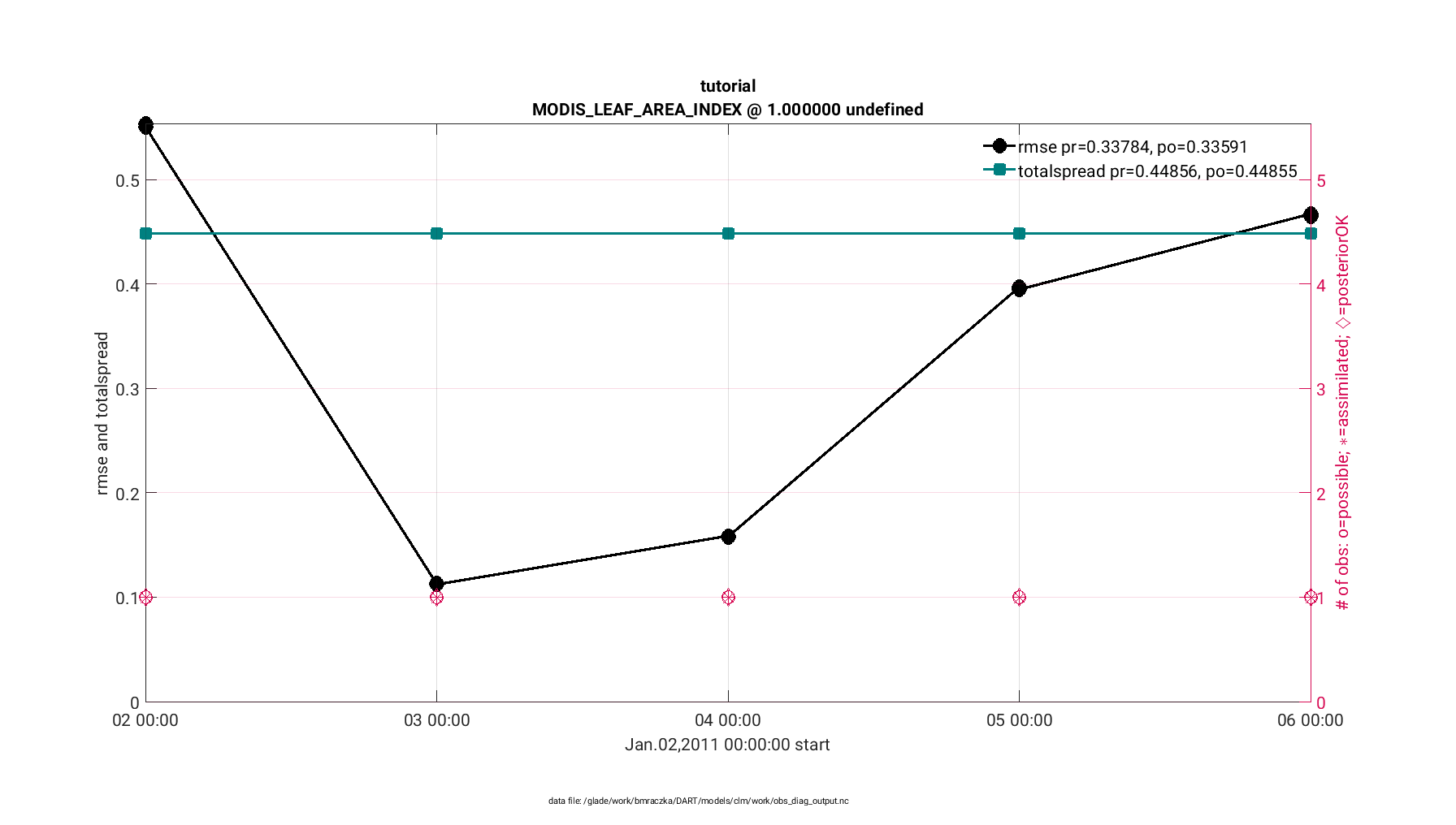
First, the plot_rmse_xxx_evolution.m script provides a time series of
assimilation statistics of 1) observation acceptance, 2) RMSE between
the observations and the expected observation (derived from the CLM state),
and 3) a third statistic of your choosing (we recommended ‘total spread’).
The observation acceptance statistic compares the number of observations assimilated versus the number of observations available for your domain. In general, it is desirable to assimilate the majority of observations that are available. The RMSE statistic quantifies the mismatch between the observations and the CLM state. A successful assimilation reduces the RMSE, thus reducing the mismatch between the observations and the CLM state. Finally the total spread provides contributions from the ensemble spread and observation error variance. This value should be comparable to the RMSE.
To execute plot_rmse_xxx_evolution.m do the following:
cd DART/models/clm/work
Confirm the DART executables used for the matlab diagnostics exist.
These should have been compiled during Step 11 of this tutorial.
The important DART executables for the diagnostics are
obs_diag and obs_seq_to_netcdf. If they do not exist,
perform the ./quickbuild.sh command to create them.
Next generate a text file that includes all the clm_obs_seq*.final
files that were created from the tutorial simulation
ls <rundir>/*final > obs_seq_files_tutorial.txt
Next edit the &obs_diag_nml namelist within the input.nml.
to assign the obs_seqence_list
to the text file containing the names of the clm_obs_seq*.final
files associated with the tutorial. Next, specify how the
observations are displayed by defining the bin settings, which
for this tutorial are set such that every day of observations
are displayed individually. Because the tutorial is a global run
we define the lonlim and latlim setting to include the
entire globe. For more information about the obs_diag namelist
settings go here.
&obs_diag_nml
  obs_sequence_name = ''
  obs_sequence_list = 'obs_seq_files_tutorial.txt'
  first_bin_center =  2011, 1,  2, 0, 0, 0
  last_bin_center  =  2011, 1,  6, 0, 0, 0
  bin_separation   =     0, 0,  1, 0, 0, 0
  bin_width        =     0, 0,  1, 0, 0, 0
  time_to_skip     =     0, 0,  0, 0, 0, 0
  max_num_bins     = 1000
  trusted_obs      = 'null'
  Nregions   = 1
  lonlim1    =     0.0,
  lonlim2    =   360.0,
  latlim1    =   -90.0,
  latlim2    =    90.0,
  reg_names  = 'tutorial',
  hlevel_edges =  0.0, 1.0, 2.0, 5.0, 10.0, 40.0
  print_mismatched_locs = .false.
  create_rank_histogram = .true.
  outliers_in_histogram = .true.
  use_zero_error_obs    = .false.
  verbose               = .true.
  /
Next convert the information in the clm_obs_seq*.final files into
a netcdf format (obs_diag_output.nc) by executing the
obs_diag executable.
./obs_diag
Next, use Matlab to create the plot_rmse_xxx_evolution.m figures.
Note that this function automatically plots the RMSE, where the copy
and the obsname variable are customizable.
cd DART/diagnostics/matlab
module load matlab
matlab -nodesktop
>> fname   = '<dartroot>/models/clm/work/obs_diag_output.nc';
>> copy    = 'totalspread';
>> obsname = 'MODIS_LEAF_AREA_INDEX';
>> plotdat = plot_rmse_xxx_evolution(fname, copy, 'obsname', obsname);
Tip
When remotely logged into Derecho there is a time delay when the Matlab figures are rendering, and also when interacting with the figures. For the purposes of this tutorial this delay is minimal. However, to improve responsiveness for your own research you may find it convenient to port your diagnostic files (e.g. obs_diag_output.nc) and run the Matlab diagnostics on your local machine. This requires a compiled version of DART and a Matlab license for your local machine.
The finished figure should look like the following below. Click on it to enlarge. Notice that the figure has two axes; the left providing the RMSE and total spread statistics, whereas the right provides the observations available and observations assimilated for each time step.
|
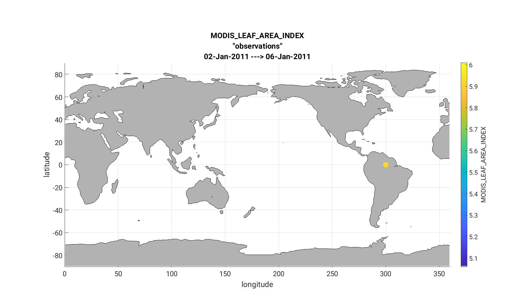
Second, the link_obs.m provides several features, including a spatial
map of the observation locations with color coded DART QC values. This allows
the user to identify observation acceptance as a function of sub-regions.
Next edit both the &obs_seq_to_netcdf_nml and &schedule_nml namelist sections
within input.nml.
For this tutorial we plot a list of the clm_obs_seq*.final files as shown below,
which includes the global domain. We include all observations within a single
bin. For more information about these settings go
here.
&obs_seq_to_netcdf_nml
  obs_sequence_name = ''
  obs_sequence_list = 'obs_seq_files_tutorial.txt'
  append_to_netcdf  = .false.
  lonlim1    =    0.0
  lonlim2    =  360.0
  latlim1    =  -90.0
  latlim2    =   90.0
  verbose    = .false.
  /

&schedule_nml
  calendar        = 'Gregorian'
  first_bin_start =  1601,  1,  1,  0,  0,  0
  first_bin_end   =  2999,  1,  1,  0,  0,  0
  last_bin_end    =  2999,  1,  1,  0,  0,  0
  bin_interval_days    = 1000000
  bin_interval_seconds = 0
  max_num_bins         = 1000
  print_table          = .true.
  /
Next execute the obs_seq_to_netcdf to convert the observation
information into a netcdf readable file (obs_epoch_001.nc) for
link_obs.m
./obs_seq_to_netcdf
Next, use Matlab to create the link_obs.m figures.
cd DART/diagnostics/matlab
module load matlab
matlab -nodesktop
>> fname         = '<dartroot>/models/clm/work/obs_epoch_001.nc';
>> ObsTypeString = 'MODIS_LEAF_AREA_INDEX';
>> ObsCopyString = 'observations';
>> CopyString    = 'prior ensemble mean';
>> QCString      = 'DART quality control';
>> region        = [0 360 -90 90 -Inf Inf];
>> global obsmat;
>> link_obs(fname, ObsTypeString, ObsCopyString, CopyString, QCString, region)
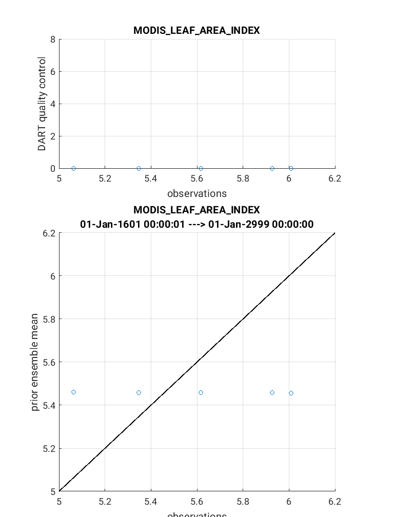
The link_obs.m script creates 3 separate figures including a 1) 3D geographic
scatterplot, 2) observation diagnostic plot as a function of time, and 3) 2D
scatterplot that typically compares the ‘prior/posterior expected obsevations’
against the ‘actual observation’. Read the commented section within the link_obs.m
script for more information.
The completed link_obs.m figures are shown below for the 3D geographic
scatterplot (left) and the 2d scatterplot (right). Click to enlarge. Note that the 2D
scatterplot compares the prior expected observations vs. the actual observations.
The 1:1 fit for this plot is poor, but should be slightly improved if you
compare the posterior observations vs. the actual observations.
Note
The matlab geographic scatterplot is rendered in 3D and can be converted into 2D
(as it appears below) by using the ‘Rotate 3D’ option at the
top of the figure or through the menu bar as Tools > Rotate 3D. Use the cursor to
rotate the map such that the vertical dimension is removed. For 3D observations with
no vertical coordinate, such as MODIS LEAF AREA, DART sets VERTISUNDEF for the
vertical coordinate and -888888 as the vertical value. During assimilation,
DART ignores the missing vertical dimension for observations with VERTISUNDEF.
For more information about specifying vertical coordinates for observations see
Creating an obs_seq file from real observations.
|
|
If you have completed all these steps (1-13) Congratulations! – you are well on your way to designing CLM5-DART assimilations for your own research.