MATLAB observation space diagnostics
Configuring MATLAB
DART uses MATLAB’s own netCDF reading and writing capability and does not use any MATLAB or third-party toolboxes.
To allow your environment to seamlessly use the DART MATLAB functions, your MATLAB path must be set to include two of the directories in the DART repository. In the MATLAB command prompt enter the following, using the real path to your DART installation:
addpath('DART/diagnostics/matlab','-BEGIN')
addpath('DART/guide/DART_LAB/matlab','-BEGIN')
It is convenient to put these commands in your ~/matlab/startup.m so they
get run every time MATLAB starts up. You can use the example startup.m file
located at DART/diagnostics/matlab/startup.m. This example startup file
contains instructions for using it.
Summary of MATLAB functions
Once you have processed the obs_seq.final files into a single
obs_diag_output.nc, you can use that as input to your own plotting routines
or use the following DART MATLAB® routines:
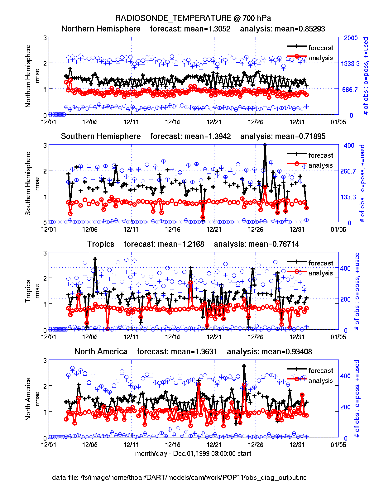
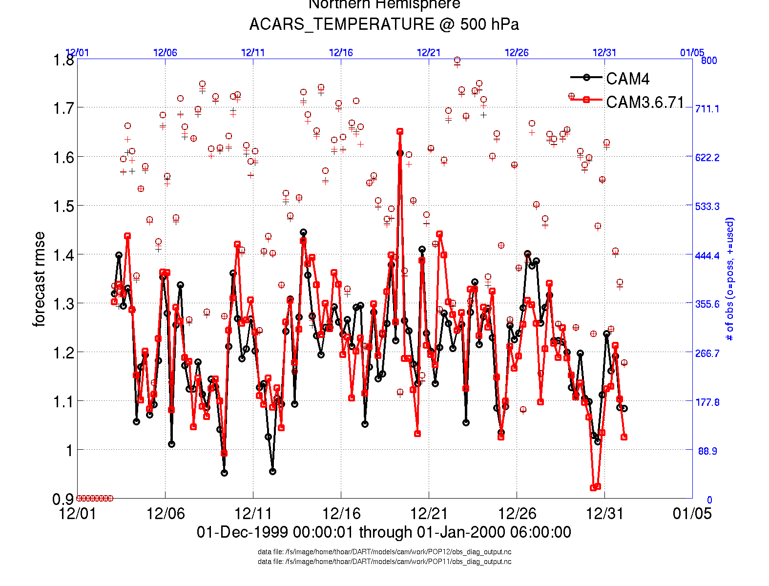
plot_evolution.m plots the temporal evolution of any of the quantities above for each variable for specified levels. The number of observations possible and used are plotted on the same axis.
fname      = 'POP11/obs_diag_output.nc';        % netcdf file produced by 'obs_diag'
copystring = 'rmse';                            % 'copy' string == quantity of interest
plotdat    = plot_evolution(fname,copystring);  % -- OR --
plotdat    = plot_evolution(fname,copystring,'obsname','RADIOSONDE_TEMPERATURE');
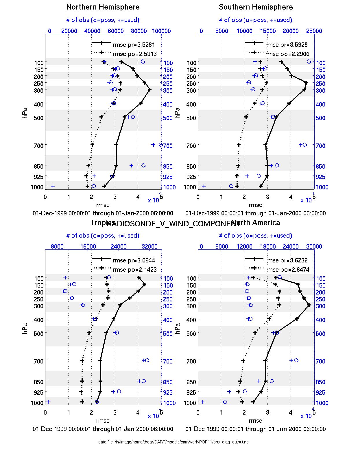
plot_profile.m plots the spatial and temporal average of any specified quantity as a function of height. The number of observations possible and used are plotted on the same axis.
fname      = 'POP11/obs_diag_output.nc';        % netcdf file produced by 'obs_diag'
copystring = 'rmse';                            % 'copy' string == quantity of interest
plotdat    = plot_profile(fname,copystring);
plot_rmse_xxx_evolution.m
same as plot_evolution.m but will overlay rmse on the same axis.
plot_rmse_xxx_profile.m
same as plot_profile.m with an overlay of rmse.
plot_bias_xxx_profile.m
same as plot_profile.m with an overlay of bias.
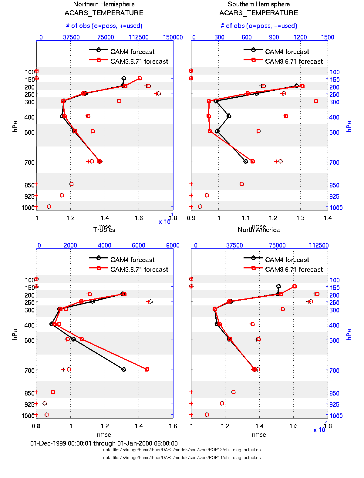
two_experiments_evolution.m
same as plot_evolution.m but will overlay multiple (more than two, actually)
experiments (i.e. multiple obs_diag_output.nc files) on the same axis. A
separate figure is created for each region in the obs_diag_output.nc file.
files    = {'POP12/obs_diag_output.nc','POP11/obs_diag_output.nc'};
titles   = {'CAM4','CAM3.6.71'};
varnames = {'ACARS_TEMPERATURE'};
qtty     = 'rmse';
prpo     = 'prior';
levelind = 5;
two_experiments_evolution(files, titles,{'ACARS_TEMPERATURE'}, qtty, prpo, levelind)
two_experiments_profile.m
same as plot_profile.m but will overlay multiple (more than two, actually)
experiments (i.e. multiple obs_diag_output.nc files) on the same axis. If
the obs_diag_output.nc file was created with multiple regions, there are
multiple axes on a single figure.
files    = {'POP12/obs_diag_output.nc','POP11/obs_diag_output.nc'};
titles   = {'CAM4','CAM3.6.71'};
varnames = {'ACARS_TEMPERATURE'};
qtty     = 'rmse';
prpo     = 'prior';
two_experiments_profile(files, titles, varnames, qtty, prpo)
plot_rank_histogram
plot_rank_histogram.m will
create rank histograms for any variable that has that information present in
obs_diag_output.nc.
fname     = 'obs_diag_output.nc'; % netcdf file produced by 'obs_diag'
timeindex = 3;                    % plot the histogram for the third timestep
plotdat   = plot_rank_histogram(fname, timeindex, 'RADIOSONDE_TEMPERATURE');
![]()
You may also convert observation sequence files to netCDF by using
PROGRAM obs_seq_to_netcdf. All
of the following routines will work on observation sequences files AFTER an
assimilation (i.e. obs_seq.final files that have been converted to netCDF),
and some of them will work on obs_seq.out-type files that have been converted.
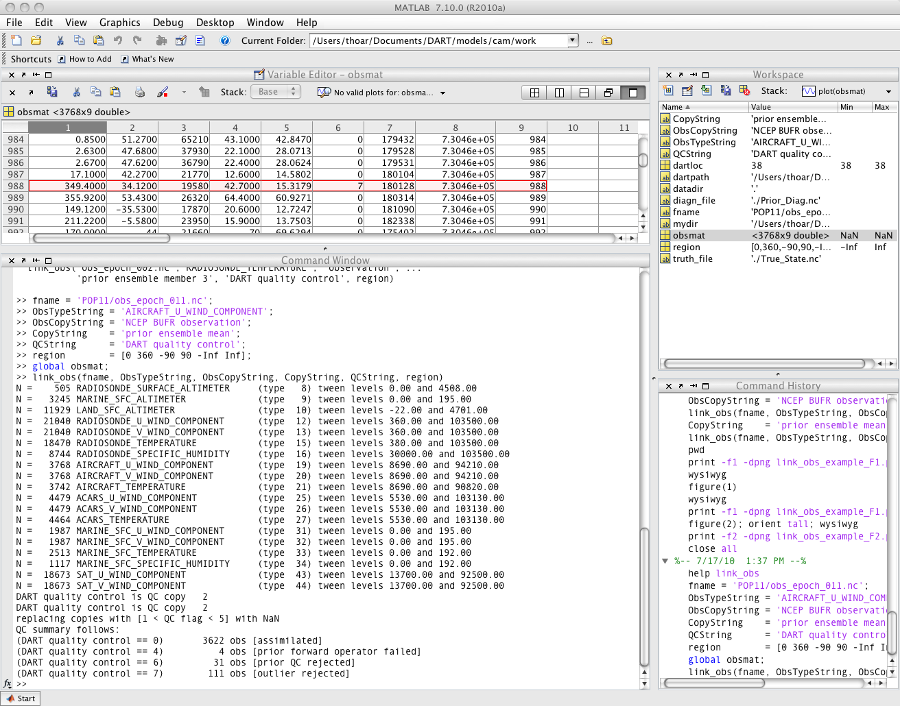
read_obs_netcdf.m reads a
particular variable and copy from a netCDF-format observation sequence file and
returns a single structure with useful bits for plotting/exploring. This routine
is the back-end for plot_obs_netcdf.m.
fname         = 'obs_sequence_001.nc';
ObsTypeString = 'RADIOSONDE_U_WIND_COMPONENT';   % or 'ALL' ...
region        = [0 360 -90 90 -Inf Inf];
CopyString    = 'NCEP BUFR observation';
QCString      = 'DART quality control';
verbose       = 1;   % anything > 0 == 'true'
obs = read_obs_netcdf(fname, ObsTypeString, region, CopyString, QCString, verbose);
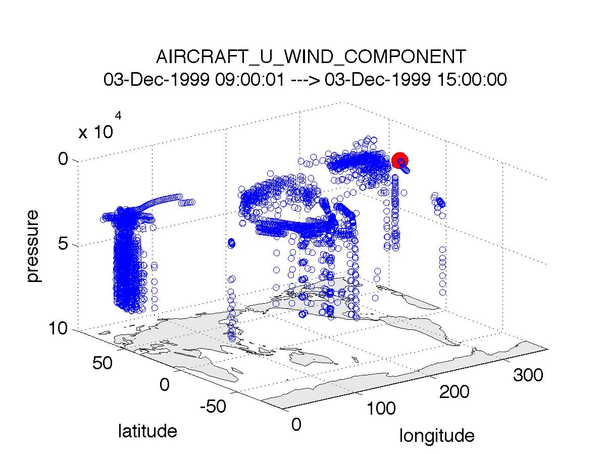
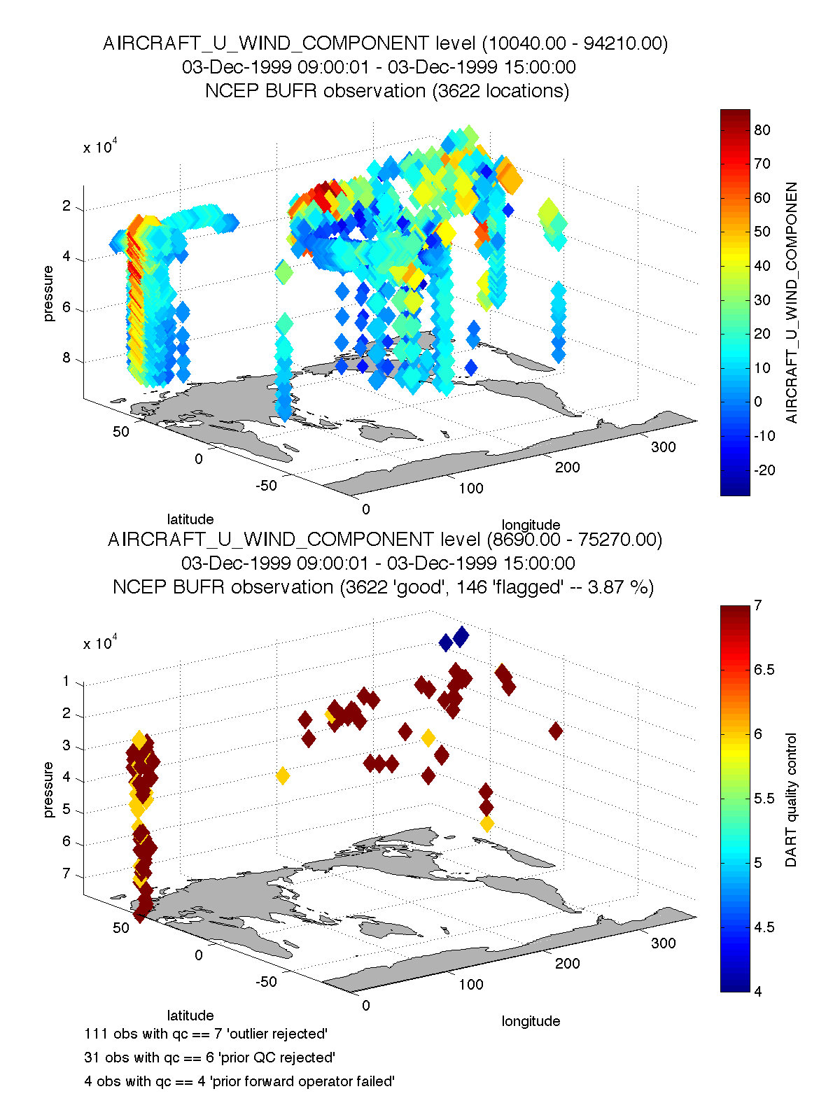
plot_obs_netcdf.m creates a 3D scatterplot of the observation locations, color-coded to the observation values. A second axis will also plot the QC values if desired.
fname         = 'POP11/obs_epoch_011.nc';
region        = [0 360 -90 90 -Inf Inf];
ObsTypeString = 'AIRCRAFT_U_WIND_COMPONENT';
CopyString    = 'NCEP BUFR observation';
QCString      = 'DART quality control';
maxgoodQC     = 2;
verbose       = 1;   % > 0 means 'print summary to command window'
twoup         = 1;   % > 0 means 'use same Figure for QC plot'
bob = plot_obs_netcdf(fname, ObsTypeString, region, CopyString, ...
                  QCString, maxgoodQC, verbose, twoup);
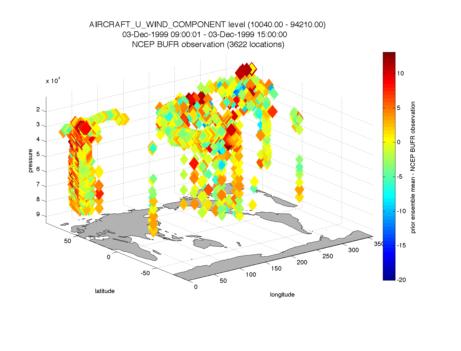
plot_obs_netcdf_diffs.m creates a 3D scatterplot of the difference between two ‘copies’ of an observation.
fname         = 'POP11/obs_epoch_011.nc';
region        = [0 360 -90 90 -Inf Inf];
ObsTypeString = 'AIRCRAFT_U_WIND_COMPONENT';
CopyString1   = 'NCEP BUFR observation';
CopyString2   = 'prior ensemble mean';
QCString      = 'DART quality control';
maxQC         = 2;
verbose       = 1;   % > 0 means 'print summary to command window'
twoup         = 0;   % > 0 means 'use same Figure for QC plot'
bob = plot_obs_netcdf_diffs(fname, ObsTypeString, region, CopyString1, CopyString2, ...
                            QCString, maxQC, verbose, twoup);
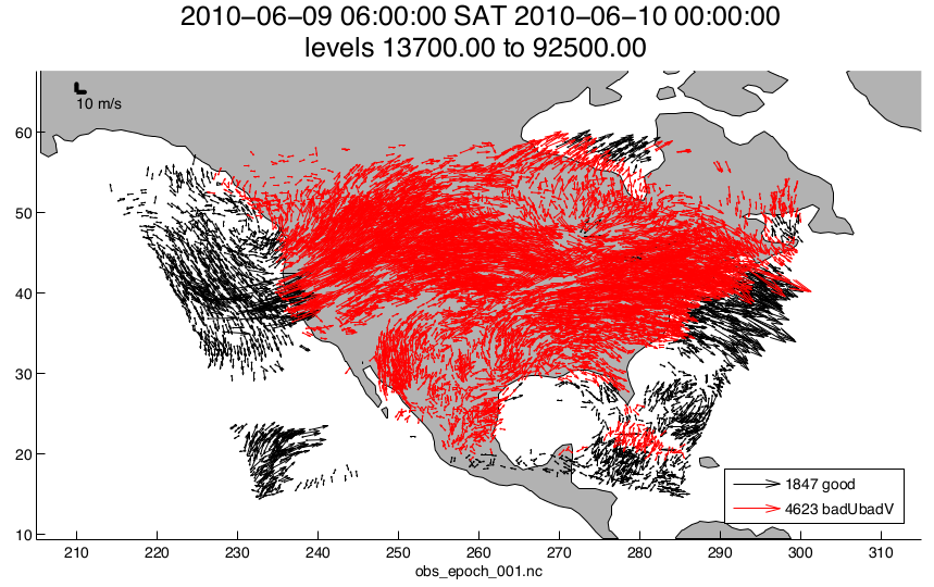
plot_wind_vectors.m
creates a 2D ‘quiver’ plot of a wind field. This function is in the
matlab/private directory - but if you want to use it, you can move it out.
I find it has very little practical value.
fname       = 'obs_epoch_001.nc';
platform    = 'SAT';    % usually 'RADIOSONDE', 'SAT', 'METAR', ...
CopyString  = 'NCEP BUFR observation';
QCString    = 'DART quality control';
region      = [210 310 12 65 -Inf Inf];
scalefactor = 5;     % reference arrow magnitude
bob = plot_wind_vectors(fname, platform, CopyString, QCString, ...
                        'region', region, 'scalefactor', scalefactor);
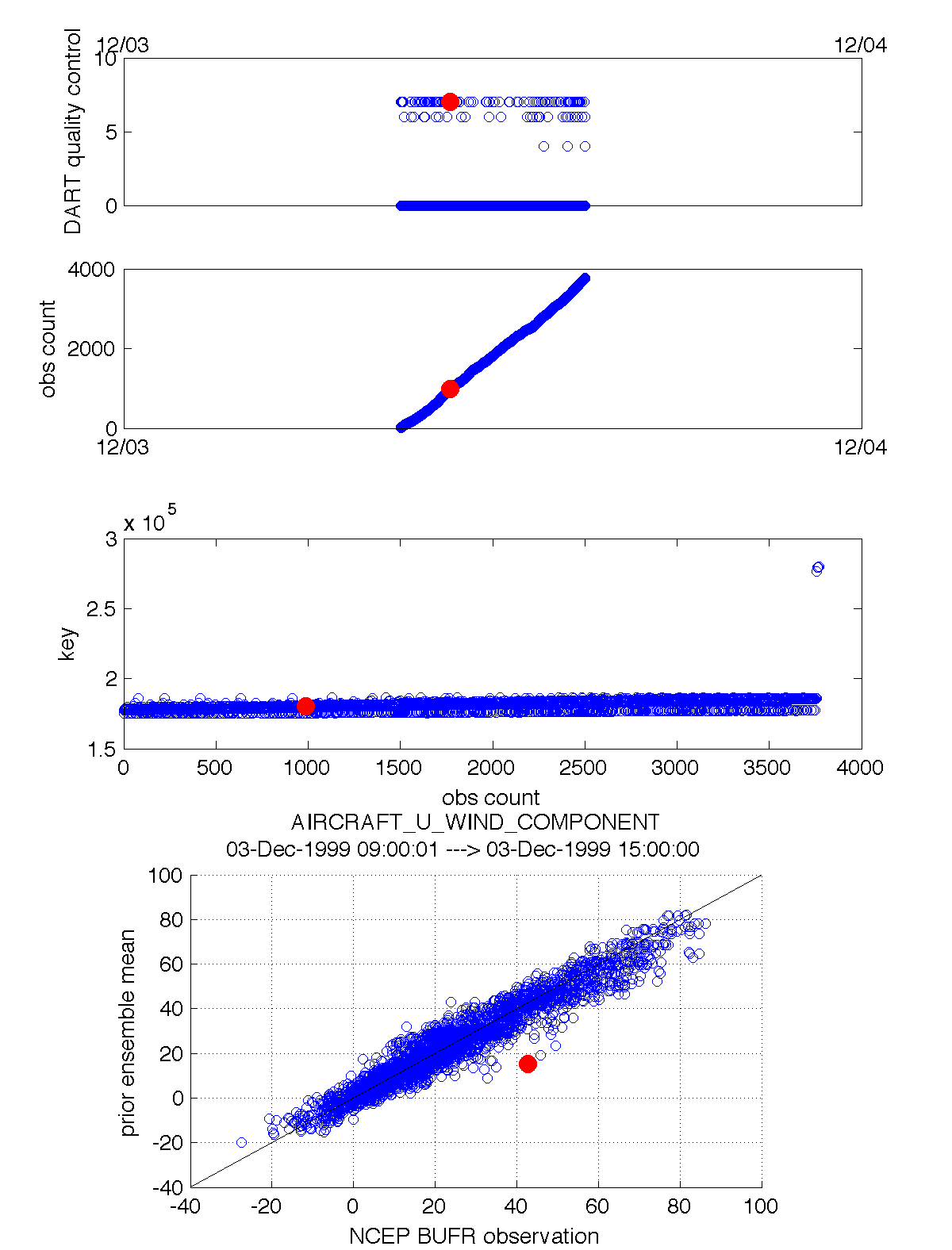
link_obs.m creates multiple figures that have linked attributes. This is my favorite function. Click on the little paintbrush icon in any of the figure frames and select some observations with “DART quality control == 7” in one window, and those same observations are highlighted in all the other windows (for example). The 3D scatterplot can be rotated around with the mouse to really pinpoint exactly where the observations are getting rejected, for example. If the data browser (the spreadsheet-like panel) is open, the selected observations get highlighted there too.
fname         = 'obs_epoch_001.nc';
ObsTypeString = 'RADIOSONDE_TEMPERATURE';
ObsCopyString = 'NCEP BUFR observation';
CopyString    = 'prior ensemble mean';
QCString      = 'DART quality control';
region        = [220 300 20 60 -Inf Inf];
global obsmat;
link_obs(fname, ObsTypeString, ObsCopyString, CopyString, QCString, region)