program obs_seq_coverage
Overview
obs_seq_coverage queries a set of observation sequence files to determine which observation locations report
frequently enough to be useful for a verification study. The big picture is to be able to pare down a large set of
observations into a compact observation sequence file to run through PROGRAM filter with all of the intended
observation types flagged as evaluate_only. DART’s forward operators then get applied and all the forecasts are
preserved in a standard obs_seq.final file - perhaps more appropriately called obs_seq.forecast! Paring down the
input observation sequence file cuts down on the unnecessary application of the forward operator to create observation
copies that will not be used anyway …
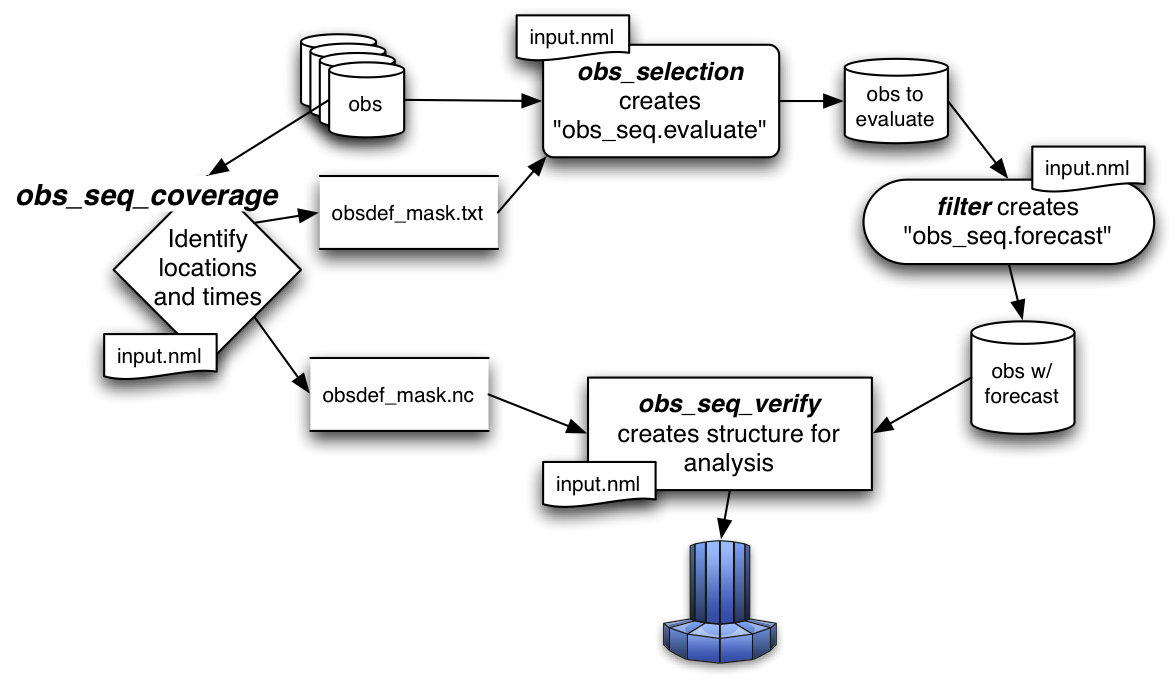
obs_seq_coverage results in two output files:
obsdef_mask.txtcontains the list of observation definitions (but not the observations themselves) that are desired. The observation definitions include the locations and times for each of the desired observation types. This file is read by program obs_selection and combined with the raw observation sequence files to create the observation sequence file appropriate for use in a forecast.obsdef_mask.nccontains information needed to be able to plot the times and locations of the observations in a manner to help explore the design of the verification locations/network.obsdef_mask.ncis required by program obs_seq_verify, the program that reorders the observations into a structure that makes it easy to calculate statistics like ROC, etc.
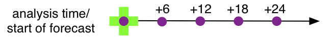
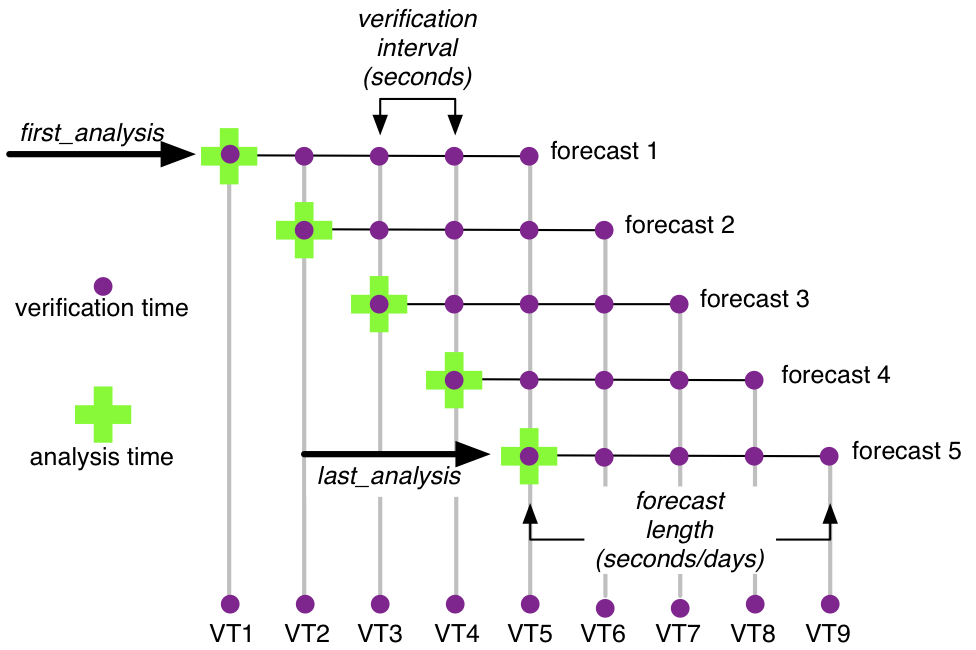
obs_seq_coverage simply provides these possible forecasts “for free”, there is no assumption
about needing them. We will use the variable verification_times to describe the complete set of times for all
possible forecasts. In our example above, there are 5 possible forecasts, each forecast consisting of 5 verification
times (the analysis time and the 4 forecast lead times). As such, there are 9 unique verification times.obs_seq_coverage.Namelist
This namelist is read from the file input.nml. Namelists start with an ampersand ‘&’ and terminate with a slash ‘/’.
Character strings that contain a ‘/’ must be enclosed in quotes to prevent them from prematurely terminating the
namelist.
&obs_seq_coverage_nml
   obs_sequences     = ''
   obs_sequence_list = ''
   obs_of_interest   = ''
   textfile_out      = 'obsdef_mask.txt'
   netcdf_out        = 'obsdef_mask.nc'
   calendar          = 'Gregorian'
   first_analysis    =  2003, 1, 1, 0, 0, 0
   last_analysis     =  2003, 1, 2, 0, 0, 0
   forecast_length_days          = 1
   forecast_length_seconds       = 0
   verification_interval_seconds = 21600
   temporal_coverage_percent     = 100.0
   lonlim1                       =  -888888.0
   lonlim2                       =  -888888.0
   latlim1                       =  -888888.0
   latlim2                       =  -888888.0
   verbose                       = .false.
   debug                         = .false.
  /
Note that -888888.0 is not a useful number. To use the defaults delete these lines from the namelist, or set them to 0.0, 360.0 and -90.0, 90.0.
The date-time integer arrays in this namelist have the form (YYYY, MM, DD, HR, MIN, SEC).
The allowable ranges for the region boundaries are: latitude [-90.,90], longitude [0.,Inf.]
You can specify either obs_sequences or obs_sequence_list – not both. One of them has to be an empty string … i.e. ‘’.
Item |
Type |
Description |
|---|---|---|
obs_sequences |
character(len=256) |
Name of the observation sequence
file(s).
This may be a relative or absolute
filename. If the filename contains a
‘/’, the filename is considered to be
comprised of everything to the right,
and a directory structure to the
left. The directory structure is then
queried to see if it can be
incremented to handle a sequence of
observation files. The default
behavior of |
obs_sequence_list |
character(len=256) |
Name of an ascii text file which contains a list of one or more observation sequence files, one per line. If this is specified, obs_sequences must be set to ‘ ‘. Can be created by any method, including sending the output of the ‘ls’ command to a file, a text editor, or another program. |
obs_of_interest |
character(len=32), dimension(:) |
These are the observation types that will be verified. It is an array of character strings that must match the standard DART observation types. Simply add as many or as few observation types as you need. Could be ‘METAR_U_10_METER_WIND’, ‘METAR_V_10_METER_WIND’,…, for example. |
textfile_out |
character(len=256) |
The name of the file that will contain the observation definitions of the verfication observations. Only the metadata from the observations (location, time, obs_type) are preserved in this file. They are in no particular order. program obs_selection will use this file as a ‘mask’ to extract the real observations from the candidate observation sequence files. |
netcdf_out |
character(len=256) |
The name of the file that will
contain the observation definitions
of the unique locations that match
any of the verification times.
This file is used in conjunction with
program obs_seq_verify
to reorder the |
calendar |
character(len=129) |
The type of the calendar used to interpret the dates. |
first_analysis |
integer, dimension(6) |
The start time of the first forecast. Also known as the analysis time of the first forecast. The six integers are: year, month, day, hour, hour, minute, second – in that order. |
last_analysis |
integer, dimension(6) |
The start time of the last forecast. The six integers are: year, month, day, hour, hour, minute, second – in that order. This needs to be a perfect multiple of the verification_interval_seconds from the start of first_analysis. |
forecast_length_days forecast_length_seconds |
integer |
both values are used to determine the total length of any single forecast. |
verification_interval_seconds |
integer |
The number of seconds between each verification.
|
temporal_coverage_percent |
real |
While it is possible to specify that you do not need an observation at every time, it makes the most sense. This is not actually required to be 100% but 100% results in the most robust comparison. |
lonlim1 |
real |
Westernmost longitude of desired region. |
lonlim2 |
real |
Easternmost longitude of desired region. If this value is less than the westernmost value, it defines a region that spans the prime meridian. It is perfectly acceptable to specify lonlim1 = 330 , lonlim2 = 50 to identify a region like “Africa”. |
latlim1 |
real |
Southernmost latitude of desired region. |
latlim2 |
real |
Northernmost latitude of desired region. |
verbose |
logical |
Print extra run-time information. |
debug |
logical |
Enable debugging messages. May generate a lot of output. |
For example:
&obs_seq_coverage_nml
   obs_sequences     = ''
   obs_sequence_list = 'obs_coverage_list.txt'
   obs_of_interest   = 'METAR_U_10_METER_WIND',
                       'METAR_V_10_METER_WIND'
   textfile_out      = 'obsdef_mask.txt'
   netcdf_out        = 'obsdef_mask.nc'
   calendar          = 'Gregorian'
   first_analysis    =  2003, 1, 1, 0, 0, 0
   last_analysis     =  2003, 1, 2, 0, 0, 0
   forecast_length_days          = 1
   forecast_length_seconds       = 0
   verification_interval_seconds = 21600
   temporal_coverage_percent     = 100.0
   lonlim1    =    0.0
   lonlim2    =  360.0
   latlim1    =  -90.0
   latlim2    =   90.0
   verbose    = .false.
   /
Other modules used
assim_model_mod
types_mod
location_mod
model_mod
null_mpi_utilities_mod
obs_def_mod
obs_kind_mod
obs_sequence_mod
random_seq_mod
time_manager_mod
utilities_mod
Files
input.nmlis used for obs_seq_coverage_nmlA text file containing the metadata for the observations to be used for forecast evaluation is created. This file is subsequently required by program obs_selection to subset the set of input observation sequence files into a single observation sequence file (
obs_seq.evaluate) for the forecast step. (obsdef_mask.txtis the default name)A netCDF file containing the metadata for a much larger set of observations that may be used is created. This file is subsequently required by program obs_seq_coverage to define the desired times and locations for the verification. (
obsdef_mask.ncis the default name)
Usage
obs_seq_coverage is built in …/DART/models/your_model/work, in the same way as the other DART components.Example: a single 48-hour forecast that is evaluated every 6 hours
obsdef_mask.txt file for a single forecast. All the required input
observation sequence filenames will be contained in a file referenced by the obs_sequence_list variable. We’ll also
restrict the observations to a specific rectangular (in Lat/Lon) region at a particular level. It is convenient to
turn on the verbose option the first time to get a feel for the logic. Here are the namelist settings if you want to
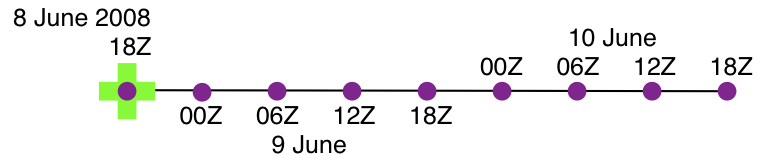
verify the METAR_U_10_METER_WIND and METAR_V_10_METER_WIND observations over the entire globe every 6 hours for 2 days
starting 18Z 8 Jun 2008:&obs_seq_coverage_nml
obs_sequences = ''
obs_sequence_list = 'obs_file_list.txt'
obs_of_interest = 'METAR_U_10_METER_WIND',
'METAR_V_10_METER_WIND'
textfile_out = 'obsdef_mask.txt'
netcdf_out = 'obsdef_mask.nc'
calendar = 'Gregorian'
first_analysis = 2008, 6, 8, 18, 0, 0
last_analysis = 2008, 6, 8, 18, 0, 0
forecast_length_days = 2
forecast_length_seconds = 0
verification_interval_seconds = 21600
temporal_coverage_percent = 100.0
lonlim1 = 0.0
lonlim2 = 360.0
latlim1 = -90.0
latlim2 = 90.0
verbose = .true.
/
The first step is to create a file containing the list of observation sequence files you want to use. This can be done with the unix command ‘ls’ with the -1 option (that’s a number one) to put one file per line, particularly if the files are organized in a nice fashion. If your observation sequence are organized like this:
/Exp1/Dir20080101/obs_seq.final
/Exp1/Dir20080102/obs_seq.final
/Exp1/Dir20080103/obs_seq.final
...
/Exp1/Dir20081231/obs_seq.final
then
ls -1 /Exp1/Dir*/obs_seq.final > obs_file_list.txt
creates the desired file. Then, simply run obs_seq_coverage - you may want to save the run-time output to a file. It
is convenient to turn on the verbose option the first time. Here is a portion of the run-time output:
[thoar@mirage2 work]$ ./obs_seq_coverage | & tee my.log
 Starting program obs_seq_coverage
 Initializing the utilities module.
 Trying to log to unit           10
 Trying to open file dart_log.out

 --------------------------------------
 Starting ... at YYYY MM DD HH MM SS =
                 2011  2 22 13 15  2
 Program obs_seq_coverage
 --------------------------------------

 set_nml_output Echo NML values to log file only
 Trying to open namelist log dart_log.nml
 location_mod: Ignoring vertical when computing distances; horizontal only
 ------------------------------------------------------


 -------------- ASSIMILATE_THESE_OBS_TYPES --------------
 RADIOSONDE_TEMPERATURE
 RADIOSONDE_U_WIND_COMPONENT
 RADIOSONDE_V_WIND_COMPONENT
 SAT_U_WIND_COMPONENT
 SAT_V_WIND_COMPONENT
 -------------- EVALUATE_THESE_OBS_TYPES --------------
 RADIOSONDE_SPECIFIC_HUMIDITY
 ------------------------------------------------------

 METAR_U_10_METER_WIND is type           36
 METAR_V_10_METER_WIND is type           37

 There are            9  verification times per forecast.
 There are            1  supported forecasts.
 There are            9  total times we need observations.

 At least           9  observations times are required at:
 verification #            1 at 2008 Jun 08 18:00:00
 verification #            2 at 2008 Jun 09 00:00:00
 verification #            3 at 2008 Jun 09 06:00:00
 verification #            4 at 2008 Jun 09 12:00:00
 verification #            5 at 2008 Jun 09 18:00:00
 verification #            6 at 2008 Jun 10 00:00:00
 verification #            7 at 2008 Jun 10 06:00:00
 verification #            8 at 2008 Jun 10 12:00:00
 verification #            9 at 2008 Jun 10 18:00:00

 obs_seq_coverage  opening obs_seq.final.2008060818
 QC index           1  NCEP QC index
 QC index           2  DART quality control

First observation time day=148812, sec=64380
First observation date 2008 Jun 08 17:53:00
 Processing obs        10000  of        84691
 Processing obs        20000  of        84691
 Processing obs        30000  of        84691
 Processing obs        40000  of        84691
 Processing obs        50000  of        84691
 Processing obs        60000  of        84691
 Processing obs        70000  of        84691
 Processing obs        80000  of        84691
 obs_seq_coverage  doneDONEdoneDONE does not exist. Finishing up.

 There were          442  voxels matching the input criterion.
...
Discussion
ASSIMILATE_THESE_OBS_TYPES and EVALUATE_THESE_OBS_TYPES are completely irrelevant -
since we’re not actually doing an assimilation. The BIG difference between the two output files is that
obsdef_mask.txt contains the metadata for just the matching observations while obsdef_mask.nc contains the
metadata for all candidate locations as well as a lot of information about the desired verification times. It is
possible to explore obsdef_mask.nc to review the selection criteria to include observations/”voxels” that do not
perfectly match the original selection criteria.obsdef_mask.nc, you can explore it with
ncdump.netcdf obsdef_mask {
dimensions:
voxel = UNLIMITED ; // (512 currently)
time = 9 ;
analysisT = 1 ;
forecast_lead = 9 ;
nlevels = 14 ;
linelen = 256 ;
nlines = 446 ;
stringlength = 32 ;
location = 3 ;
variables:
int voxel(voxel) ;
voxel:long_name = "desired voxel flag" ;
voxel:description = "1 == good voxel" ;
double time(time) ;
time:long_name = "verification time" ;
time:units = "days since 1601-1-1" ;
time:calendar = "GREGORIAN" ;
double analysisT(analysisT) ;
analysisT:long_name = "analysis (start) time of each forecast" ;
analysisT:units = "days since 1601-1-1" ;
analysisT:calendar = "GREGORIAN" ;
int forecast_lead(forecast_lead) ;
forecast_lead:long_name = "current forecast length" ;
forecast_lead:units = "seconds" ;
double verification_times(analysisT, forecast_lead) ;
verification_times:long_name = "verification times during each forecast run" ;
verification_times:units = "days since 1601-1-1" ;
verification_times:calendar = "GREGORIAN" ;
verification_times:rows = "each forecast" ;
verification_times:cols = "each verification time" ;
float mandatory_level(nlevels) ;
mandatory_level:long_name = "mandatory pressure levels" ;
mandatory_level:units = "Pa" ;
char namelist(nlines, linelen) ;
namelist:long_name = "input.nml contents" ;
char obs_type(voxel, stringlength) ;
obs_type:long_name = "observation type string at this voxel" ;
double location(voxel, location) ;
location:description = "location coordinates" ;
location:location_type = "loc3Dsphere" ;
location:long_name = "threed sphere locations: lon, lat, vertical" ;
location:storage_order = "Lon Lat Vertical" ;
location:units = "degrees degrees which_vert" ;
int which_vert(voxel) ;
which_vert:long_name = "vertical coordinate system code" ;
which_vert:VERTISUNDEF = -2 ;
which_vert:VERTISSURFACE = -1 ;
which_vert:VERTISLEVEL = 1 ;
which_vert:VERTISPRESSURE = 2 ;
which_vert:VERTISHEIGHT = 3 ;
which_vert:VERTISSCALEHEIGHT = 4 ;
int ntimes(voxel) ;
ntimes:long_name = "number of observation times at this voxel" ;
double first_time(voxel) ;
first_time:long_name = "first valid observation time at this voxel" ;
first_time:units = "days since 1601-1-1" ;
first_time:calendar = "GREGORIAN" ;
double last_time(voxel) ;
last_time:long_name = "last valid observation time at this voxel" ;
last_time:units = "days since 1601-1-1" ;
last_time:calendar = "GREGORIAN" ;
double ReportTime(voxel, time) ;
ReportTime:long_name = "time of observation" ;
ReportTime:units = "days since 1601-1-1" ;
ReportTime:calendar = "GREGORIAN" ;
ReportTime:missing_value = 0. ;
ReportTime:_FillValue = 0. ;
// global attributes:
:creation_date = "YYYY MM DD HH MM SS = 2011 03 01 09 28 40" ;
:obs_seq_coverage_source = "$URL$" ;
:obs_seq_coverage_revision = "$Revision$" ;
:obs_seq_coverage_revdate = "$Date$" ;
:min_steps_required = 9 ;
:forecast_length_days = 2 ;
:forecast_length_seconds = 0 ;
:verification_interval_seconds = 21600 ;
:obs_of_interest_001 = "METAR_U_10_METER_WIND" ;
:obs_of_interest_002 = "METAR_V_10_METER_WIND" ;
:obs_seq_file_001 = "obs_seq.final.2008060818" ;
data:
time = 148812.75, 148813, 148813.25, 148813.5, 148813.75, 148814, 148814.25,
148814.5, 148814.75 ;
forecast_lead = 0, 21600, 43200, 64800, 86400, 108000, 129600, 151200, 172800 ;
}
obsdef_mask.txt, you can run
program obs_selection to subset the observation sequence files into
one compact file to use in your ensemble forecast.References
none - but this seems like a good place to start: The Centre for Australian Weather and Climate Research - Forecast Verification Issues, Methods and FAQ