PROGRAM obs_diag (for observations that use the threed_cartesian location module)
Overview
Main program for evaluating filter performance in observation space. Primarily, the prior or posterior ensemble mean (and spread) are compared to the observation and several quantities are calculated. These quantities are then saved in a netCDF file that has all the metadata to create meaningful figures.
Each obs_seq.final file contains an observation sequence that has multiple ‘copies’ of the observation. One copy is
the actual observation, another copy is the prior ensemble mean estimate of the observation, one is the spread of the
prior ensemble estimate, one may be the prior estimate from ensemble member 1, … etc. If the original observation
sequence is the result of a ‘perfect model’ experiment, there is an additional copy called the ‘truth’ - the noise-free
expected observation given the true model state. Since this copy does not, in general, exist for the high-order models,
all comparisons are made with the copy labelled ‘observation’. There is also a namelist variable
(use_zero_error_obs) to compare against the ‘truth’ instead; the observation error variance is then automatically
set to zero.
Even with input.nml:filter_nml:num_output_obs_members set to 0; the full [prior,posterior] ensemble mean and
[prior,posterior] ensemble spread are preserved in the obs_seq.final file. Consequently, the ensemble means and
spreads are used to calculate the diagnostics. If the input.nml:filter_nml:num_output_obs_members is set to
80 (for example); the first 80 ensemble members prior and posterior “expected” values of the observation are also
included. In this case, the obs_seq.final file contains enough information to calculate a rank histograms, verify
forecasts, etc. The ensemble means are still used for many other calculations.
Since this program is fundamentally interested in the response as a function of region, there are three versions of this
program; one for each of the oned, threed_sphere, or threed_cartesian location modules (location_mod.f90). It
did not make sense to ask the lorenz_96 model what part of North America you’d like to investigate or how you would
like to bin in the vertical. The low-order models write out similar netCDF files and the Matlab scripts have been
updated accordingly. The oned observations have locations conceptualized as being on a unit circle, so only the namelist
input variables pertaining to longitude are used.
Identity observations (only possible from “perfect model experiments”) are already explored with state-space
diagnostics, so obs_diag simply skips them.
obs_diag is designed to explore the effect of the assimilation in three ways:
1) as a function of time for a particular variable and level
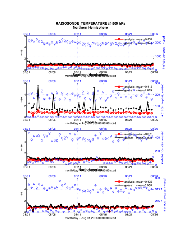
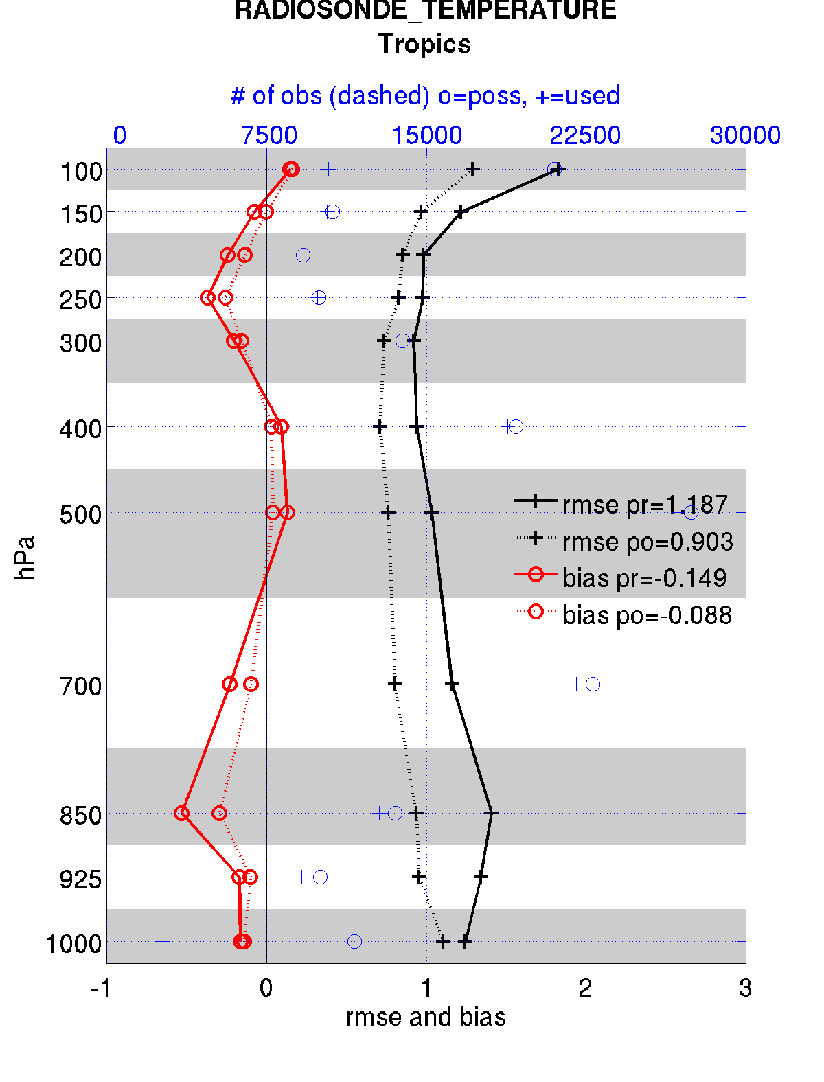
2) as a time-averaged vertical profile
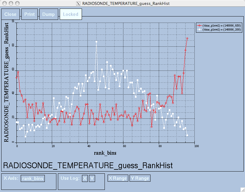
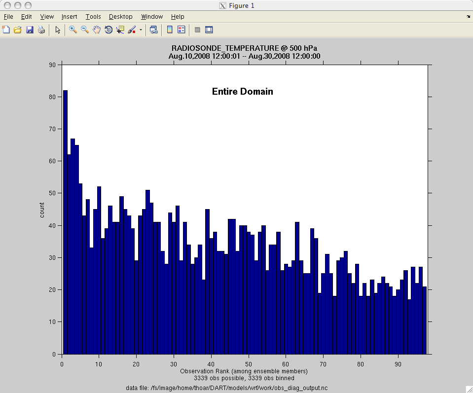
3) and in terms of a rank histogram -
“Where does the actual observation rank relative to the rest of the ensemble?”
|
|
The figures in sections 1 and 2 were created by Matlab® scripts that
query the obs_diag_output.nc file:
DART/diagnostics/matlab/plot_evolution.m and
plot_profile.m. Both of these takes as input a file name and a
‘quantity’ to plot (‘rmse’,’spread’,’totalspread’, …) and exhaustively plots
the quantity (for every variable, every level, every region) in a single matlab
figure window - and creates a series of .ps files with multiple pages for each
of the figures. The directory gets cluttered with them. The rank histogram
information in obs_diag_output.nc can easily be plotted with
ncview. (left),
a free third-party piece of software or with plot_rank_histogram.m (right).
See the Rank histograms section for more information and links to instructions.
obs_diag can be configured to compare the ensemble estimates against the ‘observation’ copy or the ‘truth’ copy
based on the setting of the use_zero_error_obs namelist variable.
The observation sequence files contain only the time of the observation, nothing of the assimilation interval, etc. - so it requires user guidance to declare what sort of temporal binning for the temporal evolution plots. I do a ‘bunch’ of arithmetic on the namelist times to convert them to a series of temporal bin edges that are used when traversing the observation sequence. The actual algorithm is that the user input for the start date and bin width set up a sequence that ends in one of two ways … the last time is reached or the number of bins has been reached.
obs_diag reads obs_seq.final files and calculates the following quantities (in no particular order) for an
arbitrary number of regions and levels. obs_diag creates a netCDF file called obs_diag_output.nc. It is
necessary to query the CopyMetaData variable to determine the storage order (i.e. “which copy is what?”) if you want
to use your own plotting routines.
ncdump -f F -v CopyMetaData obs_diag_output.nc
Nposs |
The number of observations available to be assimilated. |
Nused |
The number of observations that were assimilated. |
NbadUV |
the number of velocity observations that had a matching component that was not assimilated; |
NbadLV |
the number of observations that were above or below the highest or lowest model level, respectively; |
rmse |
The root-mean-squared error (the horizontal wind components are also used to calculate the vector wind velocity and its RMS error). |
bias |
The simple sum of forecast - observation. The bias of the horizontal wind speed (not velocity) is also computed. |
spread |
The standard deviation of the univariate obs. DART does not exploit the bivariate nature of U,V winds and so the spread of the horizontal wind is defined as the sum of the spreads of the U and V components. |
totalspread |
The total standard deviation of the estimate. We pool the ensemble variance of the observation plus the observation error variance and take the square root. |
NbadDARTQC |
the number of observations that had a DART QC value (> 1 for a prior, > 3 for a posterior) |
observation |
the mean of the observation values |
ens_mean |
the ensemble mean of the model estimates of the observation values |
N_trusted |
the number of implicitly trusted observations, regardless of DART QC |
N_DARTqc_0 |
the number of observations that had a DART QC value of 0 |
N_DARTqc_1 |
the number of observations that had a DART QC value of 1 |
N_DARTqc_2 |
the number of observations that had a DART QC value of 2 |
N_DARTqc_3 |
the number of observations that had a DART QC value of 3 |
N_DARTqc_4 |
the number of observations that had a DART QC value of 4 |
N_DARTqc_5 |
the number of observations that had a DART QC value of 5 |
N_DARTqc_6 |
the number of observations that had a DART QC value of 6 |
N_DARTqc_7 |
the number of observations that had a DART QC value of 7 |
N_DARTqc_8 |
the number of observations that had a DART QC value of 8 |
The temporal evolution of the above quantities for every observation type (RADIOSONDE_U_WIND_COMPONENT,
AIRCRAFT_SPECIFIC_HUMIDITY, …) is recorded in the output netCDF file - obs_diag_output.nc. This netCDF file can
then be loaded and displayed using the Matlab® scripts in ..../DART/diagnostics/matlab. (which may depend on
functions in ..../DART/matlab). The temporal, geographic, and vertical binning are under namelist control. Temporal
averages of the above quantities are also stored in the netCDF file. Normally, it is useful to skip the ‘burn-in’ period
- the amount of time to skip is under namelist control.
The DART QC flag is intended to provide information about whether the observation was assimilated, evaluated only, whether the assimilation resulted in a ‘good’ observation, etc. DART QC values <2 indicate the prior and posteriors are OK. DART QC values >3 were not assimilated or evaluated. Here is the table that should explain things more fully:
DART QC flag value |
meaning |
|---|---|
0 |
observation assimilated |
1 |
observation evaluated only (because of namelist settings) |
2 |
assimilated, but the posterior forward operator failed |
3 |
evaluated only, but the posterior forward operator failed |
4 |
prior forward operator failed |
5 |
not used because observation type not listed in namelist |
6 |
rejected because incoming observation QC too large |
7 |
rejected because of a failed outlier threshold test |
8 |
vertical conversion failed |
9+ |
reserved for future use |
What is new in the Manhattan release
Support for DART QC = 8 (failed vertical conversion).
Simplified input file specification.
Replace namelist integer variable
debugwith logical variableverboseto control amount of run-time output.Removed
rat_criandinput_qc_thresholdfrom the namelists. They had been deprecated for quite some time.Some of the internal variable names have been changed to make it easier to distinguish between variances and standard deviations.
What is new in the Lanai release
obs_diag has several improvements:
Improved vertical specification. Namelist variables
[h,p,m]level_edgesallow fine-grained control over the vertical binning. It is not allowed to specify both the edges and midpoints for the vertical bins.Improved error-checking for input specification, particularly the vertical bins. Repeated values are squeezed out.
Support for ‘trusted’ observations. Trusted observation types may be specified in the namelist and all observations of that type will be counted in the statistics despite the DART QC code (as long as the forward observation operator succeeds). See namelist variable
trusted_obs. For more details, see the section on Trusted observations.Support for ‘true’ observations (i.e. from an OSSE). If the ‘truth’ copy of an observation is desired for comparison (instead of the default copy) the observation error variance is set to 0.0 and the statistics are calculated relative to the ‘truth’ copy (as opposed to the normal ‘noisy’ or ‘observation’ copy). See namelist variable
use_zero_error_obs.discontinued the use of
rat_criandinput_qc_thresholdnamelist variables. Their functionality was replaced by the DART QC mechanism long ago.The creation of the rank histogram (if possible) is now namelist-controlled by namelist variable
create_rank_histogram.
Namelist
This namelist is read from the file input.nml. Namelists start with an ampersand ‘&’ and terminate with a slash ‘/’.
Character strings that contain a ‘/’ must be enclosed in quotes to prevent them from prematurely terminating the
namelist.
&obs_diag_nml
   obs_sequence_name     = ''
   obs_sequence_list     = ''
   first_bin_center      =  2003, 1, 1, 0, 0, 0
   last_bin_center       =  2003, 1, 2, 0, 0, 0
   bin_separation        =     0, 0, 0, 6, 0, 0
   bin_width             =     0, 0, 0, 6, 0, 0
   time_to_skip          =     0, 0, 0, 6, 0, 0
   max_num_bins          = 1000
   hlevel                = -888888.0
   hlevel_edges          = -888888.0
   Nregions              = 0
   xlim1                 = -888888.0
   xlim2                 = -888888.0
   ylim1                 = -888888.0
   ylim2                 = -888888.0
   reg_names             = 'null'
   trusted_obs           = 'null'
   create_rank_histogram = .true.
   outliers_in_histogram = .false.
   use_zero_error_obs    = .false.
   verbose               = .false.
   /
You can only specify either obs_sequence_name or obs_sequence_list – not both. One of them has to be an
empty string … i.e. ''.
Item |
Type |
Description |
|---|---|---|
obs_sequence_name |
character(len=256), dimension(100) |
An array of names of observation
sequence files. These may be relative
or absolute filenames. If this is
set, |
obs_sequence_list |
character(len=256) |
Name of an ascii text file which
contains a list of one or more
observation sequence files, one per
line. If this is specified,
|
first_bin_center |
integer, dimension(6) |
first timeslot of the first
obs_seq.final file to process. The
six integers are: year, month, day,
hour, hour, minute, second, in that
order. |
last_bin_center |
integer, dimension(6) |
last timeslot of interest. (reminder:
the last timeslot of day 1 is hour 0
of day 2) The six integers are: year,
month, day, hour, hour, minute,
second, in that order. This does not
need to be exact, the values from
|
bin_separation |
integer, dimension(6) |
Time between bin centers. The year and month values must be zero. |
bin_width |
integer, dimension(6) |
Time span around bin centers in which obs will be compared. The year and month values must be zero. Frequently, but not required to be, the same as the values for bin_separation. 0 |
time_to_skip |
integer, dimension(6) |
Time span at the beginning to skip
when calculating vertical profiles of
rms error and bias. The year and
month values must be zero. Useful
because it takes some time for the
assimilation to settle down from the
climatological spread at the start.
|
max_num_bins |
integer |
This provides an alternative way to
declare the |
hlevel |
real, dimension(50) |
Same, but for observations that have
height(m) or depth(m) as the vertical
coordinate. An example of defining
the midpoints is:
|
hlevel_edges |
real, dimension(51) |
The edges defining the height (or
depth) levels for the vertical
binning. You may specify either
|
Nregions |
integer |
Number of regions of the globe for
which obs space diagnostics are
computed separately. Must be between
[1,50]. If 50 is not enough, increase
|
xlim1 |
real, dimension(50) |
western extent of each of the regions. |
xlim2 |
real, dimension(50) |
eastern extent of each of the regions. |
ylim1 |
real, dimension(50) |
southern extent of the regions. |
ylim2 |
real, dimension(50) |
northern extent of the regions. |
reg_names |
character(len=129), dimension(50) |
Array of names for the regions to be analyzed. Will be used for plot titles. |
trusted_obs |
character(len=32), dimension(50) |
list of observation types that must participate in the calculation of the statistics, regardless of the DART QC (provided that the forward observation operator can still be applied without failure). e.g. ‘RADIOSONDE_TEMPERATURE’, … For more details, see the section on Trusted observations. |
use_zero_error_obs |
logical |
if |
create_rank_histogram |
logical |
if |
outliers_in_histogram |
logical |
if |
verbose |
logical |
switch controlling amount of run-time output. |
Other modules used
obs_sequence_mod
obs_kind_mod
obs_def_mod (and possibly other obs_def_xxx mods)
assim_model_mod
random_seq_mod
model_mod
location_mod
types_mod
time_manager_mod
utilities_mod
sort_mod
Files
input.nmlis used forobs_diag_nmlobs_diag_output.ncis the netCDF output filedart_log.outlist directed output from the obs_diag.LargeInnov.txtcontains the distance ratio histogram – useful for estimating the distribution of the magnitudes of the innovations.
Obs_diag may require a model input file from which to get grid information, metadata, and links to modules providing the
models expected observations. It all depends on what’s needed by the model_mod.f90
Discussion of obs_diag_output.nc
Every observation type encountered in the observation sequence file is tracked separately, and aggregated into temporal and 3D spatial bins. There are two main efforts to this program. One is to track the temporal evolution of any of the quantities available in the netCDF file for any possible observation type:
ncdump -v CopyMetaData,ObservationTypes obs_diag_output.nc
The other is to explore the vertical profile of a particular observation kind. By default, each observation kind has a ‘guess/prior’ value and an ‘analysis/posterior’ value - which shed some insight into the innovations.
Temporal evolution
The obs_diag_output.nc output file has all the metadata I could think of, as well as separate variables for every
observation type in the observation sequence file. Furthermore, there is a separate variable for the ‘guess/prior’ and
‘analysis/posterior’ estimate of the observation. To distinguish between the two, a suffix is appended to the variable
name. An example seems appropriate:
...
char CopyMetaData(copy, stringlength) ;
        CopyMetaData:long_name = "quantity names" ;
char ObservationTypes(obstypes, stringlength) ;
        ObservationTypes:long_name = "DART observation types" ;
        ObservationTypes:comment = "table relating integer to observation type string" ;
float RADIOSONDE_U_WIND_COMPONENT_guess(time, copy, hlevel, region) ;
        RADIOSONDE_U_WIND_COMPONENT_guess:_FillValue = -888888.f ;
        RADIOSONDE_U_WIND_COMPONENT_guess:missing_value = -888888.f ;
float RADIOSONDE_V_WIND_COMPONENT_guess(time, copy, hlevel, region) ;
        RADIOSONDE_V_WIND_COMPONENT_guess:_FillValue = -888888.f ;
        RADIOSONDE_V_WIND_COMPONENT_guess:missing_value = -888888.f ;
...
float MARINE_SFC_ALTIMETER_guess(time, copy, surface, region) ;
        MARINE_SFC_ALTIMETER_guess:_FillValue = -888888.f ;
        MARINE_SFC_ALTIMETER_guess:missing_value = -888888.f ;
...
float RADIOSONDE_WIND_VELOCITY_guess(time, copy, hlevel, region) ;
        RADIOSONDE_WIND_VELOCITY_guess:_FillValue = -888888.f ;
        RADIOSONDE_WIND_VELOCITY_guess:missing_value = -888888.f ;
...
float RADIOSONDE_U_WIND_COMPONENT_analy(time, copy, hlevel, region) ;
        RADIOSONDE_U_WIND_COMPONENT_analy:_FillValue = -888888.f ;
        RADIOSONDE_U_WIND_COMPONENT_analy:missing_value = -888888.f ;
float RADIOSONDE_V_WIND_COMPONENT_analy(time, copy, hlevel, region) ;
        RADIOSONDE_V_WIND_COMPONENT_analy:_FillValue = -888888.f ;
        RADIOSONDE_V_WIND_COMPONENT_analy:missing_value = -888888.f ;
...
There are several things to note:
the ‘WIND_VELOCITY’ component is nowhere ‘near’ the corresponding U,V components.
all of the ‘guess’ variables come before the matching ‘analy’ variables.
surface variables (i.e.
MARINE_SFC_ALTIMETERhave a coordinate called ‘surface’ as opposed to ‘hlevel’ for the others in this example).
Vertical profiles
Believe it or not, there are another set of netCDF variables specifically for the vertical profiles, essentially duplicating the previous variables but without the ‘time’ dimension. These are distinguished by the suffix added to the observation kind - ‘VPguess’ and ‘VPanaly’ - ‘VP’ for Vertical Profile.
...
float SAT_WIND_VELOCITY_VPguess(copy, hlevel, region) ;
        SAT_WIND_VELOCITY_VPguess:_FillValue = -888888.f ;
        SAT_WIND_VELOCITY_VPguess:missing_value = -888888.f ;
...
float RADIOSONDE_U_WIND_COMPONENT_VPanaly(copy, hlevel, region) ;
        RADIOSONDE_U_WIND_COMPONENT_VPanaly:_FillValue = -888888.f ;
        RADIOSONDE_U_WIND_COMPONENT_VPanaly:missing_value = -888888.f ;
...
Observations flagged as ‘surface’ do not participate in the vertical profiles (Because surface variables cannot exist on any other level, there’s not much to plot!). Observations on the lowest level DO participate. There’s a difference!
Rank histograms
If it is possible to calculate a rank histogram, there will also be :
...
int RADIOSONDE_U_WIND_COMPONENT_guess_RankHi(time, rank_bins, hlevel, region) ;
...
int RADIOSONDE_V_WIND_COMPONENT_guess_RankHi(time, rank_bins, hlevel, region) ;
...
int MARINE_SFC_ALTIMETER_guess_RankHist(time, rank_bins, surface, region) ;
...
as well as some global attributes. The attributes reflect the namelist settings and can be used by plotting routines to provide additional annotation for the histogram.
:DART_QCs_in_histogram = 0, 1, 2, 3, 7 ;
:outliers_in_histogram = "TRUE" ;
Please note:
netCDF restricts variable names to 40 characters, so ‘_Rank_Hist’ may be truncated.
It is sufficiently vague to try to calculate a rank histogram for a velocity derived from the assimilation of U,V components such that NO rank histogram is created for velocity. A run-time log message will inform as to which variables are NOT having a rank histogram variable preserved in the
obs_diag_output.ncfile - IFF it is possible to calculate a rank histogram in the first place.
|
|
|
“trusted” observation types
This needs to be stated up front: obs_diag is a post-processor; it cannot influence the assimilation. One
interpretation of a TRUSTED observation is that the assimilation should always use the observation, even if it is
far from the ensemble. At present (23 Feb 2015), the filter in DART does not forcibly assimilate any one observation and
selectively assimilate the others. Still, it is useful to explore the results using a set of ‘trusted type’
observations, whether they were assimilated, evaluated, or rejected by the outlier threshhold. This is the important
distinction. The diagnostics can be calculated differently for each observation type.
The normal diagnostics calculate the metrics (rmse, bias, etc.) only for the ‘good’ observations - those that were
assimilated or evaluated. The outlier_threshold essentially defines what observations are considered too far from
the ensemble prior to be useful. These observations get a DART QC of 7 and are not assimilated. The observations
with a DART QC of 7 do not contribute the the metrics being calculated. Similarly, if the forward observation operator
fails, these observations cannot contribute. When the operator fails, the ‘expected’ observation value is ‘MISSING’, and
there is no ensemble mean or spread.
‘Trusted type’ observation metrics are calculated using all the observations that were assimilated or evaluated AND
the observations that were rejected by the outlier threshhold. obs_diag can post-process the DART QC and calculate
the metrics appropriately for observation types listed in the trusted_obs namelist variable. If there are
trusted observation types specified for obs_diag, the obs_diag_output.nc has global metadata to indicate that a
different set of criteria were used to calculate the metrics. The individual variables also have an extra attribute. In
the following output, input.nml:obs_diag_nml:trusted_obs was set:
trusted_obs = 'RADIOSONDE_TEMPERATURE', 'RADIOSONDE_U_WIND_COMPONENT'
  ...
        float RADIOSONDE_U_WIND_COMPONENT_guess(time, copy, hlevel, region) ;
                RADIOSONDE_U_WIND_COMPONENT_guess:_FillValue = -888888.f ;
                RADIOSONDE_U_WIND_COMPONENT_guess:missing_value = -888888.f ;
                RADIOSONDE_U_WIND_COMPONENT_guess:TRUSTED = "TRUE" ;
        float RADIOSONDE_V_WIND_COMPONENT_guess(time, copy, hlevel, region) ;
                RADIOSONDE_V_WIND_COMPONENT_guess:_FillValue = -888888.f ;
                RADIOSONDE_V_WIND_COMPONENT_guess:missing_value = -888888.f ;
  ...
// global attributes:
  ...
                :trusted_obs_01 = "RADIOSONDE_TEMPERATURE" ;
                :trusted_obs_02 = "RADIOSONDE_U_WIND_COMPONENT" ;
                :obs_seq_file_001 = "cam_obs_seq.1978-01-01-00000.final" ;
                :obs_seq_file_002 = "cam_obs_seq.1978-01-02-00000.final" ;
                :obs_seq_file_003 = "cam_obs_seq.1978-01-03-00000.final" ;
  ...
                :MARINE_SFC_ALTIMETER = 7 ;
                :LAND_SFC_ALTIMETER = 8 ;
                :RADIOSONDE_U_WIND_COMPONENT--TRUSTED = 10 ;
                :RADIOSONDE_V_WIND_COMPONENT = 11 ;
                :RADIOSONDE_TEMPERATURE--TRUSTED = 14 ;
                :RADIOSONDE_SPECIFIC_HUMIDITY = 15 ;
                :AIRCRAFT_U_WIND_COMPONENT = 21 ;
  ...
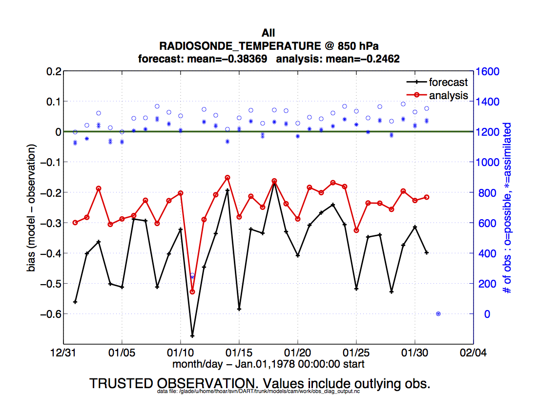
The Matlab scripts try to ensure that the trusted observation graphics clarify that the metrics plotted
are somehow ‘different’ than the normal processing stream. Some text is added to indicate that the
values include the outlying observations. IMPORTANT: The interpretation of the number of
observations ‘possible’ and ‘used’ still reflects what was used in the assimilation! The number of
observations rejected by the outlier threshhold is not explicilty plotted. To reinforce this, the text
for the observation axis on all graphics has been changed to |
|
There is ONE ambiguous case for trusted observations. There may be instances in which the observation fails the outlier
threshhold test (which is based on the prior) and the posterior forward operator fails. DART does not have a QC that
explicilty covers this case. The current logic in obs_diag correctly handles these cases except when trying to
use ‘trusted’ observations. There is a section of code in obs_diag that may be enabled if you are encountering this
ambiguous case. As obs_diag runs, a warning message is issued and a summary count is printed if the ambiguous case
is encountered. What normally happens is that if that specific observation type is trusted, the posterior values include
a MISSING value in the calculation which makes them inaccurate. If the block of code is enabled, the DART QC is recast
as the PRIOR forward observation operator fails. This is technically incorrect, but for the case of trusted
observations, it results in only calculating statistics for trusted observations that have a useful prior and posterior.
This should not be used unless you are willing to intentionally disregard ‘trusted’ observations that were rejected by
the outlier threshhold. Since the whole point of a trusted observation is to include observations potentially
rejected by the outlier threshhold, you see the problem. Some people like to compare the posteriors. THAT can be the
problem.
if ((qc_integer == 7) .and. (abs(posterior_mean(1) - MISSING_R8) < 1.0_r8)) then
            write(string1,*)'WARNING ambiguous case for obs index ',obsindex
            string2 = 'obs failed outlier threshhold AND posterior operator failed.'
            string3 = 'Counting as a Prior QC == 7, Posterior QC == 4.'
            if (trusted) then
! COMMENT      string3 = 'WARNING changing DART QC from 7 to 4'
! COMMENT      qc_integer = 4
            endif
            call error_handler(E_MSG,'obs_diag',string1,text2=string2,text3=string3)
            num_ambiguous = num_ambiguous + 1
         endif
Usage
obs_diag is built in …/DART/models/your_model/work, in the same way as the other DART components.
Multiple observation sequence files
There are two ways to specify input files for obs_diag. You can either specify the name of a file containing a list
of files (in obs_sequence_list), or you may specify a list of files via obs_sequence_name.
Example: observation sequence files spanning 30 days
In this example, we will be accumulating metrics for 30 days. The |
|
/Exp1/Dir01/obs_seq.final
/Exp1/Dir02/obs_seq.final
/Exp1/Dir03/obs_seq.final
...
/Exp1/Dir99/obs_seq.final
The first step is to create a file containing the list of observation sequence files you want to use. This can be done with the unix command ‘ls’ with the -1 option (that’s a number one) to put one file per line.
ls -1 /Exp1/Dir*/obs_seq.final > obs_file_list.txt
It is necessary to turn on the verbose option to check the first/last times that will be used for the histogram. Then, the namelist settings for 2008 07 31 12Z through 2008 08 30 12Z are:
&obs_diag_nml
   obs_sequence_name     = ''
   obs_sequence_list     = 'obs_file_list.txt'
   first_bin_center      =  2008, 8,15,12, 0, 0
   last_bin_center       =  2008, 8,15,12, 0, 0
   bin_separation        =     0, 0,30, 0, 0, 0
   bin_width             =     0, 0,30, 0, 0, 0
   time_to_skip          =     0, 0, 0, 0, 0, 0
   max_num_bins          = 1000
   Nregions              = 1
   xlim1                 = -1.0
   xlim2                 = 1000000.0
   ylim1                 = -1.0
   ylim2                 = 1000000.0
   reg_names             = 'Entire Domain'
   create_rank_histogram = .true.
   outliers_in_histogram = .false.
   verbose               = .true.
   /
then, simply run obs_diag in the usual manner - you may want to save the run-time output to a file. Here is a
portion of the run-time output:
...
Region  1 Entire Domain                    (WESN):     0.0000   360.0000   -90.0000    90.0000
 Requesting            1  assimilation periods.

epoch      1  start day=148865, sec=43201
epoch      1 center day=148880, sec=43200
epoch      1    end day=148895, sec=43200
epoch      1  start 2008 Jul 31 12:00:01
epoch      1 center 2008 Aug 15 12:00:00
epoch      1    end 2008 Aug 30 12:00:00
...
MARINE_SFC_HORIZONTAL_WIND_guess_RankHis has            0 "rank"able observations.
SAT_HORIZONTAL_WIND_guess_RankHist       has            0 "rank"able observations.
...
obs_diag_output.nc, you can explore it with plot_profile.m, plot_bias_xxx_profile.m, or
plot_rmse_xxx_profile.m,
rank histograms with ncview or plot_rank_histogram.m.References
none
Private components
N/A