PROGRAM obs_diag (for 1D observations)
Overview/usage
Main program for observation-space diagnostics for the models with 1D locations. 18 quantities are calculated for each
region for each temporal bin specified by user input. The result of the code is a netCDF file that contains the 18
quantities of the prior (aka ‘guess’) and posterior (aka ‘analysis’) estimates as a function of time and region as well
as all the metadata to create meaningful figures. The 1D version of obs_diag has defaults that automatically set
the first and last bin center based on the first and last observation time in the set of observations being processed.
This is different behavior than the 3D versions.
Each obs_seq.final file contains an observation sequence that has multiple ‘copies’ of the observation. One copy is
the actual observation, another copy is the prior ensemble mean estimate of the observation, one is the spread of the
prior ensemble estimate, one may be the prior estimate from ensemble member 1, … etc. The only observations for the 1D
models are generally the result of a ‘perfect model’ experiment, so there is an additional copy called the ‘truth’ - the
noise-free expected observation given the true model state. Since this copy does not, in general, exist for the
high-order models, all comparisons are made with the copy labelled ‘observation’. There is also a namelist variable
(use_zero_error_obs) to compare against the ‘truth’ instead; the observation error variance is then automatically
set to zero.
Even with input.nml:filter_nml:num_output_obs_members set to 0; the full [prior,posterior] ensemble mean and
[prior,posterior] ensemble spread are preserved in the obs_seq.final file. Consequently, the ensemble means and
spreads are used to calculate the diagnostics. If the input.nml:filter_nml:num_output_obs_members is set to
80 (for example); the first 80 ensemble members prior and posterior “expected” values of the observation are also
included. In this case, the obs_seq.final file contains enough information to calculate a rank histograms, verify
forecasts, etc. The ensemble means are still used for many other calculations.
|
|
Since this program is fundamentally interested in the response as a function of region, there are three versions of this
program; one for each of the oned, threed_sphere, or threed_cartesian location modules (location_mod.f90). It
did not make sense to ask the lorenz_96 model what part of North America you’d like to investigate or how you would
like to bin in the vertical. The low-order models write out similar netCDF files and the Matlab scripts have been
updated accordingly. The oned observations have locations conceptualized as being on a unit circle, so only the namelist
input variables pertaining to longitude are used.
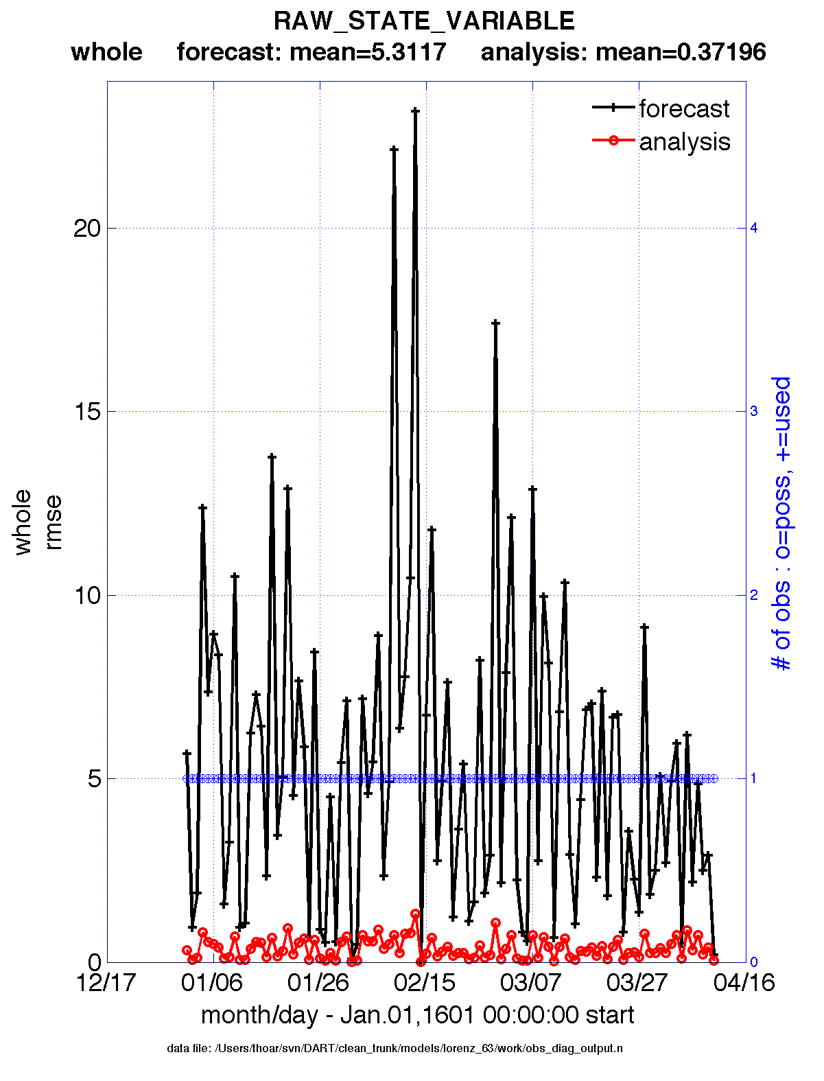
obs_diag is designed to explore the effect of the assimilation in two ways; 1) as a function of time for a
particular variable (this is the figure on the left), and sometimes 2) in terms of a rank histogram - “Where does the
actual observation rank relative to the rest of the ensemble?” (figure on the right). The figures were created by
Matlab® scripts that query the obs_diag_output.nc file:
DART/diagnostics/matlab/plot_evolution.m and
plot_rank_histogram.m. Both of these takes as input a file
name and a ‘quantity’ to plot (‘rmse’,’spread’,’totalspread’, …) and exhaustively plots the quantity (for every
variable, every region) in a single matlab figure window - and creates a series of .ps files with multiple pages for
each of the figures. The directory gets cluttered with them.
The observation sequence files contain only the time of the observation, nothing of the assimilation interval, etc. - so
it requires user guidance to declare what sort of temporal binning for the temporal evolution plots. I do a ‘bunch’ of
arithmetic on the namelist times to convert them to a series of temporal bin edges that are used when traversing the
observation sequence. The actual algorithm is that the user input for the start date and bin width set up a sequence
that ends in one of two ways … the last time is reached or the number of bins has been reached. NOTE: for the
purpose of interpretability, the 1D obs_diag routines saves ‘dates’ as GREGORIAN dates despite the fact these
systems have no concept of a calendar.
obs_diag reads obs_seq.final files and calculates the following quantities (in no particular order) for an
arbitrary number of regions and levels. obs_diag creates a netCDF file called obs_diag_output.nc. It is
necessary to query the CopyMetaData variable to determine the storage order (i.e. “which copy is what?”) if you want
to use your own plotting routines.
ncdump -f F -v CopyMetaData obs_diag_output.nc
Nposs |
The number of observations available to be assimilated. |
Nused |
The number of observations that were assimilated. |
rmse |
The root-mean-squared error (the horizontal wind components are also used to calculate the vector wind velocity and its RMS error). |
bias |
The simple sum of forecast - observation. The bias of the horizontal wind speed (not velocity) is also computed. |
spread |
The standard deviation of the univariate obs. DART does not exploit the bivariate nature of U,V winds and so the spread of the horizontal wind is defined as the sum of the spreads of the U and V components. |
totalspread |
The total standard deviation of the estimate. We pool the ensemble variance of the observation plus the observation error variance and take the square root. |
NbadDARTQC |
the number of observations that had a DART QC value (> 1 for a prior, > 3 for a posterior) |
observation |
the mean of the observation values |
ens_mean |
the ensemble mean of the model estimates of the observation values |
N_trusted |
the number of implicitly trusted observations, regardless of DART QC |
N_DARTqc_0 |
the number of observations that had a DART QC value of 0 |
N_DARTqc_1 |
the number of observations that had a DART QC value of 1 |
N_DARTqc_2 |
the number of observations that had a DART QC value of 2 |
N_DARTqc_3 |
the number of observations that had a DART QC value of 3 |
N_DARTqc_4 |
the number of observations that had a DART QC value of 4 |
N_DARTqc_5 |
the number of observations that had a DART QC value of 5 |
N_DARTqc_6 |
the number of observations that had a DART QC value of 6 |
N_DARTqc_7 |
the number of observations that had a DART QC value of 7 |
N_DARTqc_8 |
the number of observations that had a DART QC value of 8 |
The DART QC flag is intended to provide information about whether the observation was assimilated, evaluated only, whether the assimilation resulted in a ‘good’ observation, etc. DART QC values <2 indicate the prior and posteriors are OK. DART QC values >3 were not assimilated or evaluated. Here is the table that should explain things more fully:
DART QC flag value |
meaning |
|---|---|
0 |
observation assimilated |
1 |
observation evaluated only (because of namelist settings) |
2 |
assimilated, but the posterior forward operator failed |
3 |
evaluated only, but the posterior forward operator failed |
4 |
prior forward operator failed |
5 |
not used because observation type not listed in namelist |
6 |
rejected because incoming observation QC too large |
7 |
rejected because of a failed outlier threshold test |
8 |
vertical conversion failed |
9+ |
reserved for future use |
What is new in the Manhattan release
Support for DART QC = 8 (failed vertical conversion). This is provided simply to make the netCDF files as consistent as needed for plotting purposes.
Simplified input file specification.
Some of the internal variable names have been changed to make it easier to distinguish between variances and standard deviations.
What is new in the Lanai release
obs_diag has several improvements:
Support for ‘trusted’ observations. Trusted observation types may be specified in the namelist and all observations of that type will be counted in the statistics despite the DART QC code (as long as the forward observation operator succeeds). See namelist variable
trusted_obs.Support for ‘true’ observations (i.e. from an OSSE). If the ‘truth’ copy of an observation is desired for comparison (instead of the default copy) the observation error variance is set to 0.0 and the statistics are calculated relative to the ‘truth’ copy (as opposed to the normal ‘noisy’ or ‘observation’ copy). See namelist variable
use_zero_error_obs.discontinued the use of
rat_criandinput_qc_thresholdnamelist variables. Their functionality was replaced by the DART QC mechanism long ago.The creation of the rank histogram (if possible) is now namelist-controlled by namelist variable
create_rank_histogram.
Namelist
This namelist is read from the file input.nml. Namelists start with an ampersand ‘&’ and terminate with a slash ‘/’.
Character strings that contain a ‘/’ must be enclosed in quotes to prevent them from prematurely terminating the
namelist.
&obs_diag_nml
   obs_sequence_name     = ''
   obs_sequence_list     = ''
   bin_width_days        = -1
   bin_width_seconds     = -1
   init_skip_days        = 0
   init_skip_seconds     = 0
   max_num_bins          = 9999
   Nregions              = 3
   lonlim1               = 0.0, 0.0, 0.5
   lonlim2               = 1.0, 0.5, 1.0
   reg_names             = 'whole', 'yin', 'yang'
   trusted_obs           = 'null'
   use_zero_error_obs    = .false.
   create_rank_histogram = .true.
   outliers_in_histogram = .true.
   verbose               = .false.
   /
The allowable ranges for the region boundaries are: lon [0.0, 1.0). The 1D locations are conceived as the distance around a unit sphere. An observation with a location exactly ON a region boundary cannot ‘count’ for both regions. The logic used to resolve this is:
if((lon ≥ lon1) .and. (lon < lon2)) keeper = .true.
obs_sequence_name or obs_sequence_list – not both. One of them has to be
an empty string … i.e. ''.Item |
Type |
Description |
|---|---|---|
obs_sequence_name |
character(len=256), dimension(100) |
An array of names of observation
sequence files. These may be relative
or absolute filenames. If this is
set, |
obs_sequence_list |
character(len=256) |
Name of an ascii text file which
contains a list of one or more
observation sequence files, one per
line. If this is specified,
|
bin_width_days, bin_width_seconds |
integer |
Specifies the width of the analysis window. All observations within a window centered at the observation time +/- bin_width_[days,seconds] is used. If both values are 0, half the separation between observation times as defined in the observation sequence file is used for the bin width (i.e. all observations used). |
init_skip_days, init_skip_seconds |
integer |
Ignore all observations before this time. This allows one to skip the ‘spinup’ or stabilization period of an assimilation. |
max_num_bins |
integer |
This provides a way to restrict the
number of temporal bins. If
|
Nregions |
integer |
The number of regions for the unit
circle for which you’d like
observation-space diagnostics. If 3
is not enough increase |
lonlim1 |
real(r8) array of length(Nregions) |
starting value of coordinates defining ‘regions’. A value of -1 indicates the start of ‘no region’. |
lonlim2 |
real(r8) array of length(Nregions) |
ending value of coordinates defining ‘regions’. A value of -1 indicates the end of ‘no region’. |
reg_names |
character(len=6), dimension(Nregions) |
Array of names for each of the regions. The default example has the unit circle as a whole and divided into two equal parts, so there are only three regions. |
trusted_obs |
character(len=32), dimension(5) |
Array of names for observation TYPES that will be included in the statistics if at all possible (i.e. the forward observation operator succeeds). For 1D observations the only choices in the code as distributed are ‘RAW_STATE_VARIABLE’ and/or ‘RAW_STATE_1D_INTEGRAL’. (Additional 1D observation types can be added by the user.) |
use_zero_error_obs |
logical |
if |
create_rank_histogram |
logical |
if |
outliers_in_histogram |
logical |
if |
verbose |
logical |
switch controlling amount of run-time output. |
Modules directly used
types_mod
obs_sequence_mod
obs_def_mod
obs_kind_mod
location_mod
time_manager_mod
utilities_mod
sort_mod
random_seq_mod
Modules indirectly used
assim_model_mod
cov_cutoff_mod
model_mod
null_mpi_utilities_mod
Files
input.nmlis used forobs_diag_nmlobs_diag_output.ncis the netCDF output filedart_log.outlist directed output from the obs_diag.LargeInnov.txtcontains the distance ratio histogram – useful for estimating the distribution of the magnitudes of the innovations.
Discussion of obs_diag_output.nc
Every observation type encountered in the observation sequence file is tracked separately, and aggregated into temporal and spatial bins. There are two main efforts to this program. One is to track the temporal evolution of any of the quantities available in the netCDF file for any possible observation type:
ncdump -v CopyMetaData,ObservationTypes obs_diag_output.nc
The other is to explore the vertical profile of a particular observation kind. By default, each observation kind has a ‘guess/prior’ value and an ‘analysis/posterior’ value - which shed some insight into the innovations.
Temporal evolution
The obs_diag_output.nc output file has all the metadata I could think of, as well as separate variables for every
observation type in the observation sequence file. Furthermore, there is a separate variable for the ‘guess/prior’ and
‘analysis/posterior’ estimate of the observation. To distinguish between the two, a suffix is appended to the variable
name. An example seems appropriate:
...
char CopyMetaData(copy, stringlength) ;
        CopyMetaData:long_name = "quantity names" ;
...
int rank_bins(rank_bins) ;
        rank_bins:long_name = "rank histogram bins" ;
        rank_bins:comment = "position of the observation among the sorted noisy ensemble members" ;
float RAW_STATE_VARIABLE_guess(time, copy, region) ;
        RAW_STATE_VARIABLE_guess:_FillValue = -888888.f ;
        RAW_STATE_VARIABLE_guess:missing_value = -888888.f ;
float RAW_STATE_VARIABLE_analy(time, copy, region) ;
        RAW_STATE_VARIABLE_analy:_FillValue = -888888.f ;
        RAW_STATE_VARIABLE_analy:missing_value = -888888.f ;
...
Rank histograms
If it is possible to calculate a rank histogram, there will also be :
 ...
int RAW_STATE_VARIABLE_guess_RankHist(time, rank_bins, region) ;
 ...
as well as some global attributes. The attributes reflect the namelist settings and can be used by plotting routines to provide additional annotation for the histogram.
:DART_QCs_in_histogram = 0, 1, 2, 3, 7 ;
:outliers_in_histogram = "TRUE" ;
References
none
Private components
N/A