Lorenz 96 Tracer Advection
Overview
The Lorenz 96 Tracer Advection model combines the Lorenz 96 model with an upstream semi-Lagrangian method. This simulates the advection of tracer particles from any source(s) by the Lorenz 96 variables (here serving as wind).
The Lorenz 96 model was first described by Edward Lorenz during a seminar at the European Centre for Medium-Range Weather Forecasts in the Autumn of 1995, the proceedings of which were published as Lorenz (1996) [1] the following year, hence the model is commonly referred to as Lorenz 96.
Lorenz and Emmanuel (1998) [2] describe the model as:
… consisting of 40 ordinary differential equations, with the dependent variables representing values of some atmospheric quantity at 40 sites spaced equally about a latitude circle. The equations contain quadratic, linear, and constant terms representing advection, dissipation, and external forcing. Numerical integration indicates that small errors (differences between solutions) tend to double in about 2 days. Localized errors tend to spread eastward as they grow, encircling the globe after about 14 days.
We have chosen a model with \(J\) variables, denoted by:
\[X_1, ... , X_j;\]in most of our experiments we have let \(J = 40\). The governing equations are:
\[dX_j/dt=(X_{j+1}-X_{j-2})X_{j-1}-X_j+F (1)\]for:
\[j=1,...,J.\]To make Eq. (1) meaningful for all values of j we define:
\[X_{-1}=X_{J-1}, X_0=X_J, \& X_{J+1}=X_1,\]so that the variables form a cyclic chain, and may be looked at as values of some unspecified scalar meteorological quantity, perhaps vorticity or temperature, at J equally spaced sites extending around a latitude circle. Nothing will simulate the atmosphere’s latitudinal or vertical extent.
In this model we are using the Semi-Lagrangian Scheme to model how tracer particles get distributed upstream across the grids by the Lorenz 96 winds
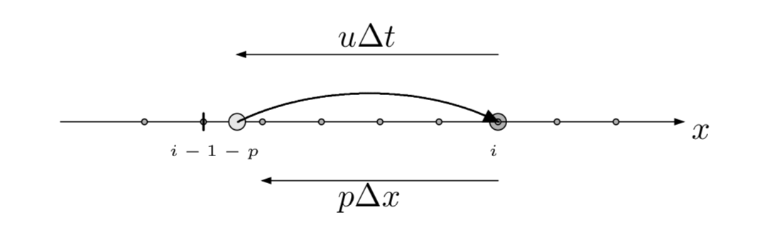
The figure above describes the implementation of the Semi-Lagrangian scheme in a one dimensional array. The tracer particle in the figure lands on a predefined grid point at tn+1. The trajectory of this tracer particle is then integrated backwards by one time step to time tn, often landing between grid points. Then, due to advection without diffusion, the concentration of tracer at time tn+1 is simply the concentration of tracer at time tn, which can be determined by interpolating concentrations of the surrounding grids [3].
Once the coupled Lorenz 96 and semi-Lagrangian is run with a source of strength 100 units/s and location at grid point one (with exponential sinks present in all grid points), the time evolution is as depicted below:
For Lorenz 96 Tracer Advection, DART advances the model, gets the model state and metadata describing this state, finds state variables that are close to a given location, and does spatial interpolation for model state variables.
Namelist
The &model_nml namelist is read from the input.nml file. Namelists
start with an ampersand & and terminate with a slash /. Character
strings that contain a / must be enclosed in quotes to prevent them from
prematurely terminating the namelist.
&model_nml
   model_size        = 120,
   forcing           = 8.00,
   delta_t           = 0.05,
   time_step_days    = 0,
   time_step_seconds = 3600
/
Description of each namelist entry
Item |
Type |
Description |
|---|---|---|
model_size |
integer |
Total number of items in the state vector. The first third of the state vector describes winds, the second third describes tracer concentration, and the final third of the state vector describes the location strength of sources. |
forcing |
real(r8) |
Forcing, F, for model. |
delta_t |
real(r8) |
Non-dimensional timestep. This is mapped to the dimensional timestep specified by time_step_days and time_step_seconds. |
time_step_days |
integer |
Number of days for dimensional timestep, mapped to delta_t. |
time_step_seconds |
integer |
Number of seconds for dimensional timestep, mapped to delta_t. |