PROGRAM obs_seq_to_netcdf
Overview
obs_seq_to_netcdf is a routine to extract the observation components from observation sequence files and write out
netCDF files that can be easily digested by other applications. This routine will allow you to plot the spatial
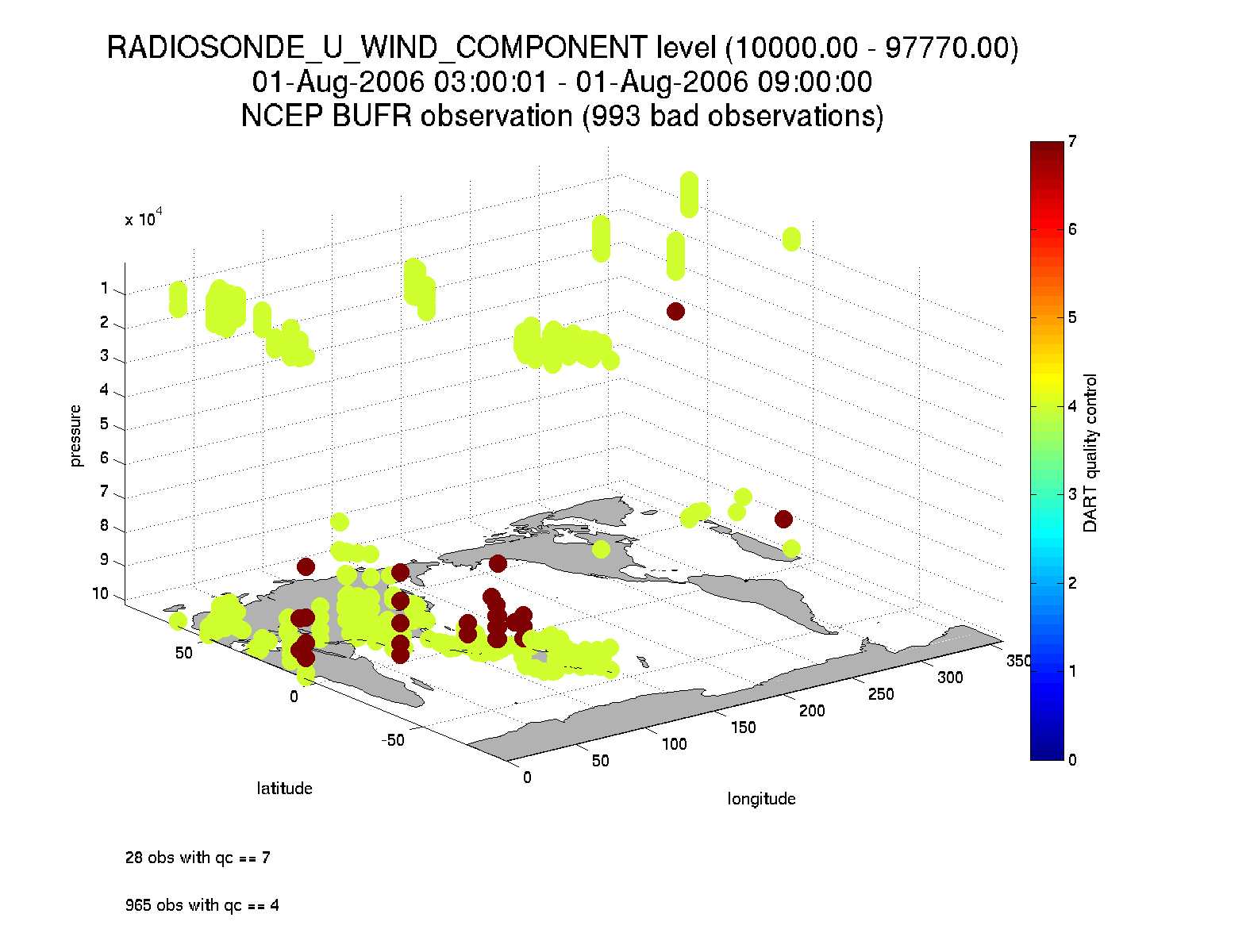
distribution of the observations and be able to discern which observations were assimilated or rejected, for example.
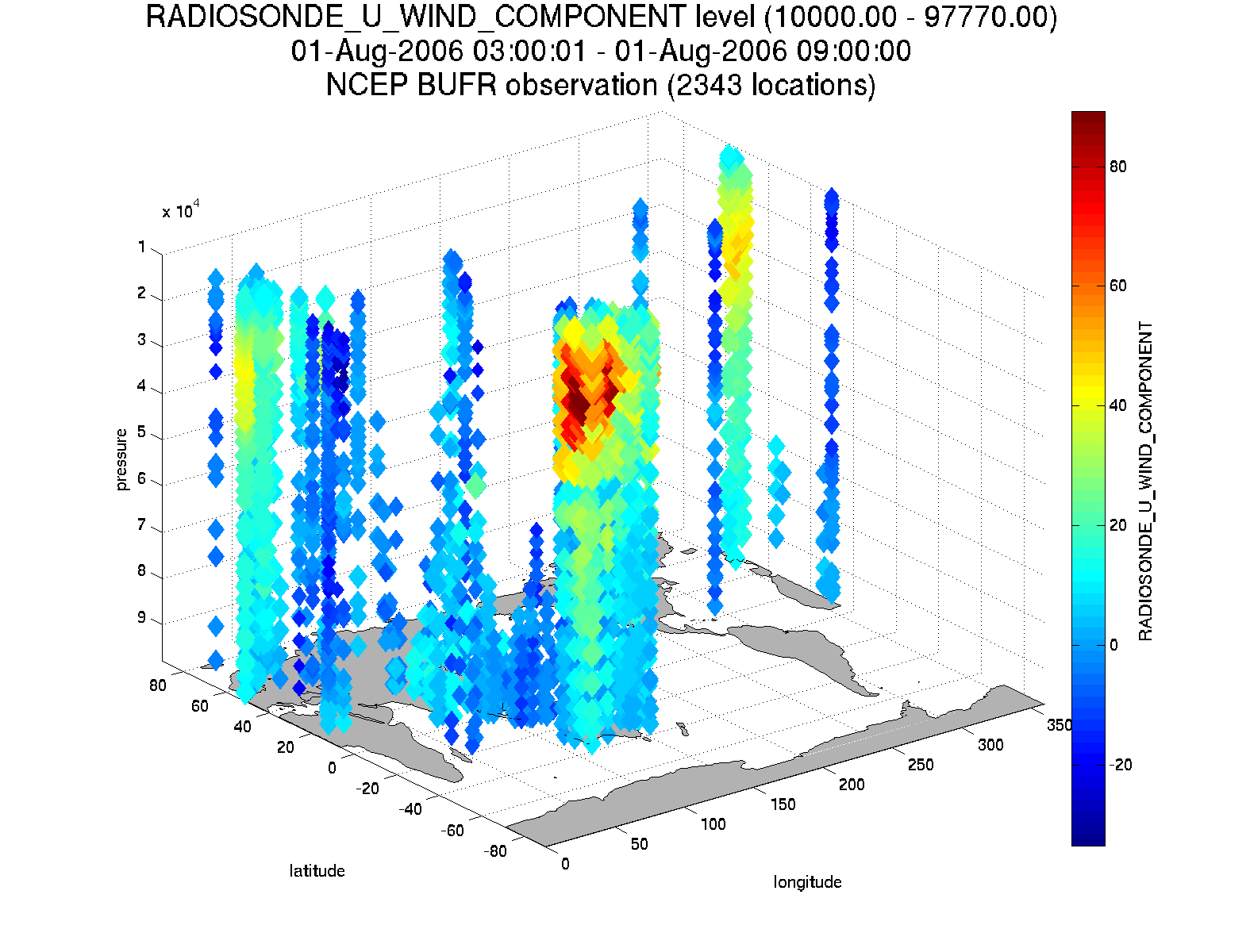
Here are some graphics from DART/diagnostics/matlab/plot_obs_netcdf.m.
The intent is that user input is queried and a series of output files - one per assimilation cycle - will contain the
observations for that cycle. It is hoped this will be useful for experiment design or, perhaps, debugging. This
routine is also the first to use the new schedule_mod module which will ultimately control the temporal aspects of
the assimilations (i.e. the assimilation schedule).
There is also a facility for exploring the spatial distributions of quantities like bias between the ensemble mean and
the observations: DART/diagnostics/matlab/plot_obs_netcdf_diffs.m.
Required namelist interfaces &obs_seq_to_netcdf and &schedule_nml are read from file input.nml.
What’s on the horizon ..
obs_seq_to_netcdf is a step toward encoding our observations in netCDF files.
The dependence on the threed_sphere/location_mod.f90 has been removed. This program will work with any
location_mod.f90. Also, this program no longer tries to construct ‘wind’ observations from horizontal components
since the program really should be faithful to preserving exactly what is in the input file. i.e. We’re not making
stuff up.
There are several Matlab scripts that understand how to read and plot observation data in netcdf format. See the
link_obs.m script that creates several linked figures with the ability to ‘brush’ data in one view and have those
selected data (and attributes) get highlighted in the other views.
Namelist
This namelist is read from the file input.nml. Namelists start with an ampersand ‘&’ and terminate with a slash ‘/’.
Character strings that contain a ‘/’ must be enclosed in quotes to prevent them from prematurely terminating the
namelist.
&obs_seq_to_netcdf_nml
   obs_sequence_name = 'obs_seq.final',
   obs_sequence_list = '',
   append_to_netcdf  = .false.,
   lonlim1    =    0.0,
   lonlim2    =  360.0,
   latlim1    =  -90.0,
   latlim2    =   90.0,
   verbose    = .false.
/
The allowable ranges for the region boundaries are: latitude [-90.,90], longitude [0.,360.] … but it is possible to
specify a region that spans the dateline by specifying the lonlim2 to be less than lonlim1.
You can only specify either obs_sequence_name or obs_sequence_list – not both.
Item |
Type |
Description |
|---|---|---|
obs_sequence_name |
character(len=256) |
Name of an observation sequence
file(s). This may be a relative or
absolute filename. If the filename
contains a ‘/’, the filename is
considered to be comprised of
everything to the right, and a
directory structure to the left. The
directory structure is then queried
to see if it can be incremented to
handle a sequence of observation
files. The default behavior of
|
obs_sequence_list |
character(len=256) |
Name of an ascii text file which contains a list of one or more observation sequence files, one per line. If this is specified, ‘obs_sequence_name’ must be set to ‘ ‘. Can be created by any method, including sending the output of the ‘ls’ command to a file, a text editor, or another program. |
append_to_netcdf |
logical |
This gives control over whether to
overwrite or append to an existing
netcdf output file. It is envisioned
that you may want to combine multiple
observation sequence files into one
netcdf file (i.e.
|
lonlim1 |
real |
Westernmost longitude of the region in degrees. |
lonlim2 |
real |
Easternmost longitude of the region
in degrees. If |
latlim1 |
real |
Southernmost latitude of the region in degrees. |
latlim2 |
real |
Northernmost latitude of the region in degrees. |
verbose |
logical |
Print extra info about the obs_seq_to_netcdf run. |
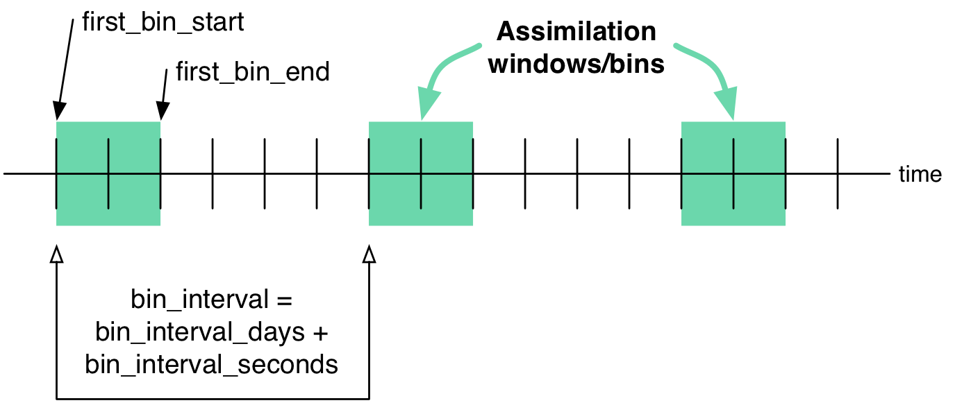
The schedule namelist
The default values specify one giant ‘bin’.
If the print_table variable is ‘true’ a summary of the assimilation schedule will be written to the screen.
&schedule_nml
   calendar       = 'Gregorian',
   first_bin_start =  1601,  1,  1,  0,  0,  0,
   first_bin_end   =  2999,  1,  1,  0,  0,  0,
   last_bin_end    =  2999,  1,  1,  0,  0,  0,
   bin_interval_days    = 1000000,
   bin_interval_seconds = 0,
   max_num_bins         = 1000,
   print_table          = .true.
  /
Item |
Type |
Description |
|---|---|---|
calendar |
character(len=32) |
Type of calendar to use to interpret dates.
May be any type supported by the
|
first_bin_start |
integer, dimension(6) |
the first time of the first assimilation period. The six integers are: year, month, day, hour, hour, minute, second – in that order. |
first_bin_end |
integer, dimension(6) |
the end of the first assimilation period. The six integers are: year, month, day, hour, hour, minute, second – in that order. |
last_bin_end |
integer, dimension(6) |
the approximate end of the last
assimilation period. The six integers are:
year, month, day, hour, hour, minute,
second – in that order. This does not need
to be exact, the values from
|
bin_interval_days, bin_interval_seconds |
integer |
Collectively, |
max_num_bins |
integer |
An alternate way to specify the maximum
number of assimilation periods. The
assimilation bin is repeated by the
bin_interval until one of two things
happens: either the last time of interest
is encountered (defined by
|
print_table |
logical |
Prints the assimilation schedule. |
Example
The following example illustrates the fact the last_bin_end does not have to be a ‘perfect’ bin end - and it gives
you an idea of an assimilation schedule table. Note that the user input defines the last bin to end at 09 Z, but the
last bin in the table ends at 06 Z.
&schedule_nml
   calendar        = 'Gregorian',
   first_bin_start =  2006, 8, 1, 0, 0, 0 ,
   first_bin_end   =  2006, 8, 1, 6, 0, 0 ,
   last_bin_end    =  2006, 8, 2, 9, 0, 0 ,
   bin_interval_days    = 0,
   bin_interval_seconds = 21600,
   max_num_bins         = 1000,
   print_table          = .true.
   /
This is the ‘table’ part of the run-time output:
Requesting  5  assimilation periods.

epoch      1  start day=148135, sec=1
epoch      1    end day=148135, sec=21600
epoch      1  start 2006 Aug 01 00:00:01
epoch      1    end 2006 Aug 01 06:00:00

epoch      2  start day=148135, sec=21601
epoch      2    end day=148135, sec=43200
epoch      2  start 2006 Aug 01 06:00:01
epoch      2    end 2006 Aug 01 12:00:00

epoch      3  start day=148135, sec=43201
epoch      3    end day=148135, sec=64800
epoch      3  start 2006 Aug 01 12:00:01
epoch      3    end 2006 Aug 01 18:00:00

epoch      4  start day=148135, sec=64801
epoch      4    end day=148136, sec=0
epoch      4  start 2006 Aug 01 18:00:01
epoch      4    end 2006 Aug 02 00:00:00

epoch      5  start day=148136, sec=1
epoch      5    end day=148136, sec=21600
epoch      5  start 2006 Aug 02 00:00:01
epoch      5    end 2006 Aug 02 06:00:00
Notice that the leading edge of an assimilation window/bin/epoch/period is actually 1 second after the specified start time. This is consistent with the way DART has always worked. If you specify assimilation windows that fully occupy the temporal continuum, there has to be some decision at the edges. An observation precisely ON the edge should only participate in one assimilation window. Historically, DART has always taken observations precisely on an edge to be part of the subsequent assimilation cycle. The smallest amount of time representable to DART is 1 second, so the smallest possible delta is added to one of the assimilation edges.
Other modules used
location_mod
netcdf
obs_def_mod
obs_kind_mod
obs_sequence_mod
schedule_mod
time_manager_mod
typeSizes
types_mod
utilities_mod
Naturally, the program must be compiled with support for the observation types contained in the observation sequence
files, so preprocess must be run to build appropriate obs_def_mod and obs_kind_mod modules - which may need
specific obs_def_?????.f90 files.
Files
Run-time
input.nmlis used forobs_seq_to_netcdf_nmlandschedule_nml.obs_epoch_xxx.ncis a netCDF output file for assimilation period ‘xxx’. Each observation copy is preserved - as are any/all QC values/copies.dart_log.outlist directed output from the obs_seq_to_netcdf.
Discussion of obs_epoch_xxx.nc structure
This might be a good time to review the basic observation sequence file structure. The only thing missing in the netcdf files is the ‘shared’ metadata for observations (e.g. GPS occultations). The observation locations, values, qc flags, error variances, etc., are all preserved in the netCDF files. The intent is to provide everything you need to make sensible plots of the observations. Some important aspects are highlighted.
[shad] % ncdump -v QCMetaData,CopyMetaData,ObsTypesMetaData obs_epoch_001.nc
netcdf obs_epoch_001 {
dimensions:
        linelen = 129 ;
        nlines = 104 ;
        stringlength = 32 ;
        copy = 7 ;
        qc_copy = 2 ;
        location = 3 ;
        ObsTypes = 58 ;
        ObsIndex = UNLIMITED ; // (4752 currently)
variables:
        int copy(copy) ;
                copy:explanation = "see CopyMetaData" ;
        int qc_copy(qc_copy) ;
                qc_copy:explanation = "see QCMetaData" ;
        int ObsTypes(ObsTypes) ;
                ObsTypes:explanation = "see ObsTypesMetaData" ;
        char ObsTypesMetaData(ObsTypes, stringlength) ;
                ObsTypesMetaData:long_name = "DART observation types" ;
                ObsTypesMetaData:comment = "table relating integer to observation type string" ;
        char QCMetaData(qc_copy, stringlength) ;
                QCMetaData:long_name = "quantity names" ;
        char CopyMetaData(copy, stringlength) ;
                CopyMetaData:long_name = "quantity names" ;
        char namelist(nlines, linelen) ;
                namelist:long_name = "input.nml contents" ;
        int ObsIndex(ObsIndex) ;
                ObsIndex:long_name = "observation index" ;
                ObsIndex:units = "dimensionless" ;
        double time(ObsIndex) ;
                time:long_name = "time of observation" ;
                time:units = "days since 1601-1-1" ;
                time:calendar = "GREGORIAN" ;
                time:valid_range = 1.15740740740741e-05, 0.25 ;
        int obs_type(ObsIndex) ;
                obs_type:long_name = "DART observation type" ;
                obs_type:explanation = "see ObsTypesMetaData" ;
                location:units = "deg_Lon deg_Lat vertical" ;
        double observations(ObsIndex, copy) ;
                observations:long_name = "org observation, estimates, etc." ;
                observations:explanation = "see CopyMetaData" ;
                observations:missing_value = 9.96920996838687e+36 ;
        int qc(ObsIndex, qc_copy) ;
                qc:long_name = "QC values" ;
                qc:explanation = "see QCMetaData" ;
        double location(ObsIndex, location) ;
                location:long_name = "location of observation" ;
                location:storage_order = "Lon Lat Vertical" ;
                location:units = "degrees degrees which_vert" ;
        int which_vert(ObsIndex) ;
                which_vert:long_name = "vertical coordinate system code" ;
                which_vert:VERTISUNDEF = -2 ;
                which_vert:VERTISSURFACE = -1 ;
                which_vert:VERTISLEVEL = 1 ;
                which_vert:VERTISPRESSURE = 2 ;
                which_vert:VERTISHEIGHT = 3 ;

// global attributes:
                :creation_date = "YYYY MM DD HH MM SS = 2009 05 01 16 51 18" ;
                :obs_seq_to_netcdf_source = "$url: http://subversion.ucar.edu/DAReS/DART/trunk/obs_sequence/obs_seq_to_netcdf.f90 $" ;
                :obs_seq_to_netcdf_revision = "$revision: 4272 $" ;
                :obs_seq_to_netcdf_revdate = "$date: 2010-02-12 14:26:40 -0700 (Fri, 12 Feb 2010) $" ;
                :obs_seq_file_001 = "bgrid_solo/work/01_01/obs_seq.final" ;
data:

 ObsTypesMetaData =
  "RADIOSONDE_U_WIND_COMPONENT     ",
  "RADIOSONDE_V_WIND_COMPONENT     ",
  "RADIOSONDE_SURFACE_PRESSURE     ",
  "RADIOSONDE_TEMPERATURE          ",
  "RADIOSONDE_SPECIFIC_HUMIDITY    ",
  ...
  yeah, yeah, yeah ... we're very impressed ...
  ...
  "VORTEX_PMIN                     ",
  "VORTEX_WMAX                     " ;

 QCMetaData =
  "Quality Control                 ",
  "DART quality control            " ;

 CopyMetaData =
  "observations                    ",
  "truth                           ",
  "prior ensemble mean             ",
  "posterior ensemble mean         ",
  "prior ensemble spread           ",
  "posterior ensemble spread       ",
  "observation error variance      " ;
}
ObsIndex. The observations variable is a 2D array - each column is a ‘copy’ of the observation. The
interpretation of the column is found in the CopyMetaData variable. Same thing goes for the qc variable - each
column is defined by the QCMetaData variable.Obs_Type variable is crucial. Each observation has an integer code to define the specific … DART observation
type. In our example - lets assume that observation number 10 (i.e. ObsIndex == 10) has an obs_type of 3 [i.e.
obs_type(10) = 3]. Since ObsTypesMetaData(3) == "RADIOSONDE_SURFACE_PRESSURE", we know that any/all quantities
where ObsIndex == 10 pertain to a radiosonde surface pressure observation.Usage
Obs_seq_to_netcdf example
&schedule_nml
   calendar        = 'Gregorian',
   first_bin_start =  2006, 8, 1, 3, 0, 0 ,
   first_bin_end   =  2006, 8, 1, 9, 0, 0 ,
   last_bin_end    =  2006, 8, 3, 3, 0, 0 ,
   bin_interval_days    = 0,
   bin_interval_seconds = 21600,
   max_num_bins         = 1000,
   print_table          = .true.
   /

&obs_seq_to_netcdf_nml
   obs_sequence_name = '',
   obs_sequence_list = 'olist',
   append_to_netcdf  = .false.,
   lonlim1    =    0.0,
   lonlim2    =  360.0,
   latlim1    =  -80.0,
   latlim2    =   80.0,
   verbose    = .false.
   /

> cat olist
/users/thoar/temp/obs_0001/obs_seq.final
/users/thoar/temp/obs_0002/obs_seq.final
/users/thoar/temp/obs_0003/obs_seq.final
Here is the pruned run-time output. Note that multiple input observation sequence files are queried and the routine ends (in this case) when the first observation time in a file is beyond the last time of interest.
 --------------------------------------
 Starting ... at YYYY MM DD HH MM SS =
                 2009  5 15  9  0 23
 Program obs_seq_to_netcdf
 --------------------------------------

 Requesting            8  assimilation periods.

epoch      1  start day=148135, sec=10801
epoch      1    end day=148135, sec=32400
epoch      1  start 2006 Aug 01 03:00:01
epoch      1    end 2006 Aug 01 09:00:00

epoch      2  start day=148135, sec=32401
epoch      2    end day=148135, sec=54000
epoch      2  start 2006 Aug 01 09:00:01
epoch      2    end 2006 Aug 01 15:00:00

epoch      3  start day=148135, sec=54001
epoch      3    end day=148135, sec=75600
epoch      3  start 2006 Aug 01 15:00:01
epoch      3    end 2006 Aug 01 21:00:00

epoch      4  start day=148135, sec=75601
epoch      4    end day=148136, sec=10800
epoch      4  start 2006 Aug 01 21:00:01
epoch      4    end 2006 Aug 02 03:00:00

epoch      5  start day=148136, sec=10801
epoch      5    end day=148136, sec=32400
epoch      5  start 2006 Aug 02 03:00:01
epoch      5    end 2006 Aug 02 09:00:00

epoch      6  start day=148136, sec=32401
epoch      6    end day=148136, sec=54000
epoch      6  start 2006 Aug 02 09:00:01
epoch      6    end 2006 Aug 02 15:00:00

epoch      7  start day=148136, sec=54001
epoch      7    end day=148136, sec=75600
epoch      7  start 2006 Aug 02 15:00:01
epoch      7    end 2006 Aug 02 21:00:00

epoch      8  start day=148136, sec=75601
epoch      8    end day=148137, sec=10800
epoch      8  start 2006 Aug 02 21:00:01
epoch      8    end 2006 Aug 03 03:00:00

 obs_seq_to_netcdf  opening /users/thoar/temp/obs_0001/obs_seq.final

 num_obs_in_epoch (           1 ) =       103223
 InitNetCDF  obs_epoch_001.nc is fortran unit            5
 num_obs_in_epoch (           2 ) =       186523
 InitNetCDF  obs_epoch_002.nc is fortran unit            5
 num_obs_in_epoch (           3 ) =       110395
 InitNetCDF  obs_epoch_003.nc is fortran unit            5
 num_obs_in_epoch (           4 ) =       191957
 InitNetCDF  obs_epoch_004.nc is fortran unit            5

 obs_seq_to_netcdf  opening /users/thoar/temp/obs_0002/obs_seq.final

 num_obs_in_epoch (           5 ) =        90683
 InitNetCDF  obs_epoch_005.nc is fortran unit            5
 num_obs_in_epoch (           6 ) =       186316
 InitNetCDF  obs_epoch_006.nc is fortran unit            5
 num_obs_in_epoch (           7 ) =       109465
 InitNetCDF  obs_epoch_007.nc is fortran unit            5
 num_obs_in_epoch (           8 ) =       197441
 InitNetCDF  obs_epoch_008.nc is fortran unit            5

 obs_seq_to_netcdf  opening /users/thoar/temp/obs_0003/obs_seq.final

 --------------------------------------
 Finished ... at YYYY MM DD HH MM SS =
                 2009  5 15  9  2 56
 --------------------------------------
Matlab setup
DART/diagnostics/matlab functions available to Matlab,
so be sure your MATLABPATH is set such that you have access to plot_obs_netcdf>> addpath('replace_this_with_the_real_path_to/DART/diagnostics/matlab')
plot_obs_netcdf and
plot_obs_netcdf_diffs are available by using the Matlab ‘help’ facility (i.e. help plot_obs_netcdf ). A quick
discussion of them here still seems appropriate. If you run the following Matlab commands with an
obs_sequence_001.nc file you cannot possibly have:>> help plot_obs_netcdf
fname = 'obs_sequence_001.nc';
ObsTypeString = 'RADIOSONDE_U_WIND_COMPONENT';
region = [0 360 -90 90 -Inf Inf];
CopyString = 'NCEP BUFR observation';
QCString = 'DART quality control';
maxQC = 2;
verbose = 1;
obs = plot_obs_netcdf(fname, ObsTypeString, region, CopyString, QCString, maxQC, verbose);
>> fname = 'obs_sequence_001.nc';
>> ObsTypeString = 'RADIOSONDE_U_WIND_COMPONENT';
>> region = [0 360 -90 90 -Inf Inf];
>> CopyString = 'NCEP BUFR observation';
>> QCString = 'DART quality control';
>> maxQC = 2;
>> verbose = 1;
>> obs = plot_obs_netcdf(fname, ObsTypeString, region, CopyString, QCString, maxQC, verbose);
N = 3336 RADIOSONDE_U_WIND_COMPONENT obs (type 1) between levels 550.00 and 101400.00
N = 3336 RADIOSONDE_V_WIND_COMPONENT obs (type 2) between levels 550.00 and 101400.00
N = 31 RADIOSONDE_SURFACE_PRESSURE obs (type 3) between levels 0.00 and 1378.00
N = 1276 RADIOSONDE_TEMPERATURE obs (type 4) between levels 550.00 and 101400.00
N = 691 RADIOSONDE_SPECIFIC_HUMIDITY obs (type 5) between levels 30000.00 and 101400.00
N = 11634 AIRCRAFT_U_WIND_COMPONENT obs (type 6) between levels 17870.00 and 99510.00
N = 11634 AIRCRAFT_V_WIND_COMPONENT obs (type 7) between levels 17870.00 and 99510.00
N = 8433 AIRCRAFT_TEMPERATURE obs (type 8) between levels 17870.00 and 76710.00
N = 6993 ACARS_U_WIND_COMPONENT obs (type 10) between levels 17870.00 and 76680.00
N = 6993 ACARS_V_WIND_COMPONENT obs (type 11) between levels 17870.00 and 76680.00
N = 6717 ACARS_TEMPERATURE obs (type 12) between levels 17870.00 and 76680.00
N = 20713 SAT_U_WIND_COMPONENT obs (type 22) between levels 10050.00 and 99440.00
N = 20713 SAT_V_WIND_COMPONENT obs (type 23) between levels 10050.00 and 99440.00
N = 723 GPSRO_REFRACTIVITY obs (type 46) between levels 220.00 and 12000.00
NCEP BUFR observation is copy 1
DART quality control is copy 2
Removing 993 obs with a DART quality control value greater than 2.000000
QCMetaData and
CopyMetaData, respectively. If you’re not so keen on a 3D plot, simply change the view to be directly ‘overhead’:>> view(0,90)
And if you act today, we’ll throw in a structure containing the selected data AT NO EXTRA CHARGE.
>> obs
obs =
            fname: 'obs_sequence_001.nc'
    ObsTypeString: 'RADIOSONDE_U_WIND_COMPONENT'
           region: [0 360 -90 90 -Inf Inf]
       CopyString: 'NCEP BUFR observation'
         QCString: 'DART quality control'
            maxQC: 2
          verbose: 1
             lons: [2343x1 double]
             lats: [2343x1 double]
                z: [2343x1 double]
              obs: [2343x1 double]
             Ztyp: [2343x1 double]
               qc: [2343x1 double]
         numbadqc: 993
           badobs: [1x1 struct]
If there are observations with QC values above that defined by maxQC there will be a badobs structure as a
component in the obs structure.
References
none
Private components
N/A