Data assimilation in DART using the Lorenz 63 model
In this section we open the “black box” of the Lorenz model that was previously used in Compiling DART. This section assumes you have successfully run the Lorenz 63 model with the example observation files that were distributed with the DART repository. In this section you will learn in more detail how DART interacts with the Lorenz 63 model to perform data assimilation.
The input.nml namelist
The DART/models/lorenz_63/work/input.nml file is the Lorenz model
namelist, which is a standard Fortran method for passing parameters from a
text file into a program without needing to recompile. There are many sections
within this file that drive the behavior of DART while using the Lorenz 63 model
for assimilation. Within input.nml, there is a section called model_nml,
which contains the model-specific parameters:
&model_nml
   sigma  = 10.0,
   r      = 28.0,
   b      = 2.6666666666667,
   deltat = 0.01,
   time_step_days = 0,
   time_step_seconds = 3600,
   solver = 'RK2'
   /
Here, you can see the values for the parameters sigma, r, and b that
were discussed in the previous section. These are the original values Lorenz
used in the 1963 paper to create the classic butterfly attractor.
The Lorenz 63 model code
The Lorenz 63 model code, which is under
DART/models/lorenz_63/model_mod.f90, contains the lines:
subroutine comp_dt(x, dt)

real(r8), intent( in) ::  x(:)
real(r8), intent(out) :: dt(:)

! compute the lorenz model dt from standard equations

dt(1) = sigma * (x(2) - x(1))
dt(2) = -x(1)*x(3) + r*x(1) - x(2)
dt(3) = x(1)*x(2) - b*x(3)

end subroutine comp_dt
which directly translates the above ODE into Fortran.
Note that the routine comp_dt does not explicitly depend on the time
variable, only on the state variables (i.e. the Lorenz 63 model is time
invariant).
Note
By default, the model_mod.f90 follows the Lorenz 63 paper to use the
Runge-Kutta 2 scheme (otherwise known as RK2 or the midpoint scheme) to
advance the model.
Since the Lorenz 63 model is time invariant, the RK2 code to advance the ODE in
time can be written as follows, again following the Lorenz 63 paper, for a
fract fraction of a time-step (typically equal to 1):
!------------------------------------------------------------------
!> does single time step advance for lorenz convective 3 variable model
!> using two step rk time step

subroutine adv_single(x, fract)

real(r8), intent(inout) :: x(:)
real(r8), intent(in)    :: fract

real(r8) :: x1(3), x2(3), dx(3)

call comp_dt(x, dx)            !  compute the first intermediate step
x1 = x + fract * deltat * dx

call comp_dt(x1, dx)           !  compute the second intermediate step
x2 = x1 + fract * deltat * dx

!  new value for x is average of original value and second intermediate

x = (x + x2) / 2.0_r8

end subroutine adv_single
Together, these two code blocks describe how the Lorenz 63 model is advanced in time. You will see how DART uses this functionality shortly.
The model time step and length of the data assimilation
In the original Lorenz 63 paper, the model is run for 50 “days” using a non-dimensional time-step of 0.01, which is reproduced in the namelist above. This time-step was assumed equal to 3600 seconds, or one hour, in dimensional time. This is also set in the namelist above. The Lorenz 63 model observation file included with the DART repository uses observations of all three state variables every six hours (so every six model steps) to conduct the assimilation.
If you were previously able to run the Matlab diagnostic scripts, you may have noticed that the butterfly attractor for the included example does not look as smooth as might be desired:
This is because the model output was only saved once every six “hours” at the observation times. As an exercise, let’s make a nicer-looking plot using the computational power available today, which even on the most humble of computers is many times greater than what Lorenz had in 1963. Let’s change Lorenz’s classic experiment to the following:
Make the non-dimensional timestep 0.001, a factor of 10 smaller, which will correspond to a dimensional timestep of 360 seconds (6 minutes). This smaller time-step will lead to a smoother model trajectory.
Keep the original ratio of time steps to observations included in the DART repository of assimilating observations every six time steps, meaning we now need observations every 36 minutes.
Therefore, in order to conduct our new experiment, we will need to regenerate the DART observation sequence files.
To change the time-step, change the input.nml file in
DART/models/lorenz_63/work to the following:
&model_nml
   sigma  = 10.0,
   r      = 28.0,
   b      = 2.6666666666667,
   deltat = 0.001,
   time_step_days = 0,
   time_step_seconds = 360
   /
Note
The changes are to deltat and time_step_seconds. Additionally:
you do not need to recompile the DART code as the purpose of namelist files
is to pass run-time parameters to a Fortran program without recompilation.
Updating the observation sequence
Let’s now regenerate the DART observation files with the updated timestep and observation ratio. In a typical large-scale application, the user will provide observations to DART in a standardized format called the Observation Sequence file. Since there are no real observations of the Lorenz 63 system, we must create our own synthetic observations - which may be done using create_obs_sequence, create_fixed_network_seq, and perfect_model_obs programs; each of which we will explain below. These helpful interactive programs are included with DART to generate these observation sequence files for typical research or education-oriented experiments. In such setups, observations (with noise added) will be generated at regular intervals from a model “truth”. This “truth” will only be available to the experiment through the noisy observations but can later be used for comparison purposes. The number of steps necessary for the ensemble members to reach the true model state’s “attractor” can be investigated and, for example, compared between different DA methods. This is an example of an “OSSE” — see High-level data assimilation workflows in DART for more information.
The three programs used in this example to create an observation sequence again are create_obs_sequence, create_fixed_network_seq, and perfect_model_obs. create_obs_sequence creates a template for the observations, create_fixed_network_seq repeats that template at multiple times, and finally perfect_model_obs harvests the observation values. These programs have many additional capabilities; if interested, see the corresponding program’s documentation.
Let’s now run the DART program create_obs_sequence to create the observation template that we will later replicate in time:
# Make sure you are in the DART/models/lorenz_63/work directory ./create_obs_sequence
The program create_obs_sequence will ask for the number of observations. Since we plan to have 3 observations at each time step (one for each of the state variables), input 3:
set_nml_output Echo NML values to log file only

--------------------------------------------------------
-------------- ASSIMILATE_THESE_OBS_TYPES --------------
  RAW_STATE_VARIABLE
--------------------------------------------------------
-------------- EVALUATE_THESE_OBS_TYPES   --------------
  none
--------------------------------------------------------
---------- USE_PRECOMPUTED_FO_OBS_TYPES   --------------
  none
--------------------------------------------------------

Input upper bound on number of observations in sequence
3
For this experimental setup, we will not have any additional copies of the data, nor will we have any quality control fields. So use 0 for both.
Input number of copies of data (0 for just a definition)
0
Input number of quality control values per field (0 or greater)
0
We now will setup each of the three observations. The program asks to enter -1 if there are no additional observations, so input anything else instead (1 below). Then enter -1, -2, and -3 in sequence for the state variable index (the observation here is just the values of the state variable). Use 0 0 for the time (we will setup a regularly repeating observation after we finish this), and 8 for the error variance for each observation.
Finally, after inputting press enter to use the default output file
set_def.out.
Input your values as follows:
input a -1 if there are no more obs
1
    Input -1 * state variable index for identity observations
    OR input the name of the observation kind from table below:
    OR input the integer index, BUT see documentation...
               1 RAW_STATE_VARIABLE
-1
input time in days and seconds (as integers)
0 0
Input the error variance for this observation definition
8
input a -1 if there are no more obs
1
    Input -1 * state variable index for identity observations
    OR input the name of the observation kind from table below:
    OR input the integer index, BUT see documentation...
               1 RAW_STATE_VARIABLE
-2
input time in days and seconds (as integers)
0 0
Input the error variance for this observation definition
8
input a -1 if there are no more obs
1
    Input -1 * state variable index for identity observations
    OR input the name of the observation kind from table below:
    OR input the integer index, BUT see documentation...
               1 RAW_STATE_VARIABLE
-3
input time in days and seconds (as integers)
0 0
Input the error variance for this observation definition
8
Input filename for sequence (<return> for set_def.out )

write_obs_seq  opening formatted observation sequence file "set_def.out"
write_obs_seq  closed observation sequence file "set_def.out"
create_obs_sequence Finished successfully.
Creating a regular sequence of observations
We will now utilize another DART program that takes this set_def.out file as
input. The interactive program create_fixed_network_seq is a helper tool
that can be used to generate a DART observation sequence file made of a set of
regularly repeating observations.
# Make sure you are in the DART/models/lorenz_63/work directory ./create_fixed_network_seq
We want to use the default set_def.out file, so press return. We also want a
regularly repeating time sequence, so input 1.
set_nml_output Echo NML values to log file only

--------------------------------------------------------
-------------- ASSIMILATE_THESE_OBS_TYPES --------------
  RAW_STATE_VARIABLE
--------------------------------------------------------
-------------- EVALUATE_THESE_OBS_TYPES   --------------
  none
--------------------------------------------------------
---------- USE_PRECOMPUTED_FO_OBS_TYPES   --------------
  none
--------------------------------------------------------

Input filename for network definition sequence (<return> for set_def.out  )

To input a regularly repeating time sequence enter 1
To enter an irregular list of times enter 2
1
We now will input the number of observations in the file. The purpose of this exercise is to refine the time step used by Lorenz in 1963 by a factor of 10. Since we want to keep the ratio of six model steps per observation and run for 50 days, we will need 2000 model observations (360 seconds × 6 × 2000 = 50 days).
As we specified in set_def.out, there are 3 observations per time step,
so a total of 6000 observations will be generated.
Note
The Lorenz 63 model dimensional time-step is related to the observational
time only through this mechanism. In other words, deltat in the
namelist could relate to virtually any dimensional time step
time_step_seconds if the observation times were not considered. However,
DART will automatically advance the model state to the observation times in
order to conduct the data assimilation at the appropriate time, then repeat
this process until no additional observations are available, thus indirectly
linking deltat to time_step_seconds.
Enter 2000 for the number of observation times. The initial time will be 0 0, and the input period will be 0 days and 2160 seconds (36 minutes).
Input number of observation times in sequence
2000
Input initial time in sequence
input time in days and seconds (as integers)
0 0
Input period of obs in sequence in days and seconds
0 2160
The numbers 1 to 2000 will then be output by create_fixed_network_seq. Press
return to accept the default output name of obs_seq.in. The file suffix is
.in as this will be the input to the next program, perfect_model_obs.
   1
   2
...
1998
1999
2000
What is output file name for sequence (<return> for obs_seq.in)

  write_obs_seq  opening formatted observation sequence file "obs_seq.in"
  write_obs_seq  closed observation sequence file "obs_seq.in"
  create_fixed_network_seq Finished successfully.
Running perfect_model_obs
We are now ready to run perfect_model_obs, which will read in obs_seq.in
and generate the observations as well as create the “perfect” model trajectory.
“Perfect” here is a synonym for the known “true” state which is used to generate
the observations. Once noise is added (to represent observational uncertainty),
the output is written to obs_seq.out.
# Make sure you are in the DART/models/lorenz_63/work directory./perfect_model_obs
The output should look like the following:
set_nml_output Echo NML values to log file only
 initialize_mpi_utilities: Running single process

--------------------------------------------------------
-------------- ASSIMILATE_THESE_OBS_TYPES --------------
   RAW_STATE_VARIABLE
--------------------------------------------------------
-------------- EVALUATE_THESE_OBS_TYPES   --------------
   none
--------------------------------------------------------
---------- USE_PRECOMPUTED_FO_OBS_TYPES   --------------
   none
--------------------------------------------------------

 quality_control_mod: Will reject obs with Data QC larger than    3
 quality_control_mod: No observation outlier threshold rejection will be done
 perfect_main  Model size =                     3
 perfect_read_restart: reading input state from file
 perfect_main  total number of obs in sequence is         6000
 perfect_main  number of qc values is            1

 perfect_model_obs: Main evaluation loop, starting iteration    0
 move_ahead Next assimilation window starts    at:  day=       0 sec=     0
 move_ahead Next assimilation window ends      at:  day=       0 sec=   180
 perfect_model_obs: Model does not need to run; data already at required time
 perfect_model_obs: Ready to evaluate up to       3 observations

 perfect_model_obs: Main evaluation loop, starting iteration    1
 move_ahead Next assimilation window starts    at:  day=       0 sec=  1981
 move_ahead Next assimilation window ends      at:  day=       0 sec=  2340
 perfect_model_obs: Ready to run model to advance data ahead in time
 perfect_model_obs: Ready to evaluate up to       3 observations

...

perfect_model_obs: Main evaluation loop, starting iteration 1999
move_ahead Next assimilation window starts    at:  day=      49 sec= 84061
move_ahead Next assimilation window ends      at:  day=      49 sec= 84420
perfect_model_obs: Ready to run model to advance data ahead in time
perfect_model_obs: Ready to evaluate up to       3 observations

perfect_model_obs: Main evaluation loop, starting iteration 2000
perfect_model_obs: No more obs to evaluate, exiting main loop
perfect_model_obs: End of main evaluation loop, starting cleanup
write_obs_seq  opening formatted observation sequence file "obs_seq.out"
write_obs_seq  closed observation sequence file "obs_seq.out"
You can now see the files true_state.nc, a netCDF file which has the perfect
model state at all 2000 observation times; obs_seq.out, an ASCII file which
contains the 6000 observations (2000 times with 3 observations each) of the true
model state with noise added in; and perfect_output.nc, a netCDF file with
the final true state that could be used to “restart” the experiment from the
final time (49.75 days in this case).
We can now see the relationship between obs_seq.in and obs_seq.out:
obs_seq.in contains a “template” of the desired observation locations and
types, while obs_seq.out is a list of the actual observation values, in this
case generated by the perfect_model_obs program.
Important
create_obs_seq is used for this low-order model because there are no
real observations for Lorenz 63. For systems that have real observations,
DART provides a variety of observation converters available to convert
from native observation formats to the DART format. See
Available observation converter programs for a list.
Running the filter
Now that obs_seq.out and true_state.nc have been prepared, DART can
perform the actual data assimilation. This will generate an ensemble of model
states, use the ensemble to estimate the prior distribution, compare to the
“expected” observation of each member, and update the model state according to
Bayes’ rule.
# Make sure you are in the DART/models/lorenz_63/work directory ./filter
set_nml_output Echo NML values to log file only
initialize_mpi_utilities: Running single process

--------------------------------------------------------
-------------- ASSIMILATE_THESE_OBS_TYPES --------------
  RAW_STATE_VARIABLE
--------------------------------------------------------
-------------- EVALUATE_THESE_OBS_TYPES   --------------
  none
--------------------------------------------------------
---------- USE_PRECOMPUTED_FO_OBS_TYPES   --------------
  none
--------------------------------------------------------

quality_control_mod: Will reject obs with Data QC larger than    3
quality_control_mod: No observation outlier threshold rejection will be done
assim_tools_init: Selected filter type is Ensemble Adjustment Kalman Filter (EAKF)
assim_tools_init: The cutoff namelist value is     1000000.000000
assim_tools_init: ... cutoff is the localization half-width parameter,
assim_tools_init: ... so the effective localization radius is     2000000.000000
filter_main: running with an ensemble size of    20
parse_stages_to_write:  filter will write stage : preassim
parse_stages_to_write:  filter will write stage : analysis
parse_stages_to_write:  filter will write stage : output
set_member_file_metadata no file list given for stage "preassim" so using default names
set_member_file_metadata no file list given for stage "analysis" so using default names
Prior inflation: None
Posterior inflation: None
filter_main: Reading in initial condition/restart data for all ensemble members from file(s)

filter: Main assimilation loop, starting iteration    0
move_ahead Next assimilation window starts    at:  day=       0 sec=     0
move_ahead Next assimilation window ends      at:  day=       0 sec=   180
filter: Model does not need to run; data already at required time
filter: Ready to assimilate up to       3 observations
comp_cov_factor: Standard Gaspari Cohn localization selected
filter_assim: Processed       3 total observations

filter: Main assimilation loop, starting iteration    1
move_ahead Next assimilation window starts    at:  day=       0 sec= 21421
move_ahead Next assimilation window ends      at:  day=       0 sec= 21780
filter: Ready to run model to advance data ahead in time
filter: Ready to assimilate up to       3 observations
filter_assim: Processed       3 total observations
...

filter: Main assimilation loop, starting iteration  199
move_ahead Next assimilation window starts    at:  day=      49 sec= 64621
move_ahead Next assimilation window ends      at:  day=      49 sec= 64980
filter: Ready to run model to advance data ahead in time
filter: Ready to assimilate up to       3 observations
filter_assim: Processed       3 total observations

filter: Main assimilation loop, starting iteration  200
filter: No more obs to assimilate, exiting main loop
filter: End of main filter assimilation loop, starting cleanup
write_obs_seq  opening formatted observation sequence file "obs_seq.final"
write_obs_seq  closed observation sequence file "obs_seq.final"
Based on the default Lorenz 63 input.nml namelist for filter included in
the DART repository, the assimilation will have three stages:
The preassim stage, where the ensemble is updated by advancing the model. The file
preassim.nc, which contains the pre-assimilation model trajectories for all the ensemble members, will be written.The analysis stage, where the data assimilation is conducted. The post-assimilation model trajectories for all the ensemble members will be written to
analysis.ncThe output stage, which writes the file
obs_seq.finalcontaining the actual observations as assimilated plus the ensemble forward-operator expected values and any quality-control values. This stage also writes thefilter_output.ncfile containing the ensemble state from the final cycle, which could be used to restart the experiment.
DART has now successfully assimilated our updated observations with a 6 minute model time step and assimilation every 36 minutes. :tada:
Verifying the nicer-looking results
You can now run the verification scripts (as in the section Verifying installation) in Matlab with the following commands:
>> addpath ../../../diagnostics/matlab>> plot_ens_time_series
Some additional commands to view the attractor from the ZY plane were used:
>> set(findall(gca, ‘Type’, ‘Line’),‘LineWidth’,2);>> set(gca,‘FontSize’,18)>> xlabel(‘x’)>> ylabel(‘y’)>> zlabel(‘z’)>> view([90 0])
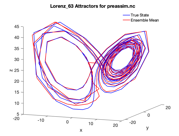
We can now see the following smooth Lorenz 63 true state and ensemble mean comparison with a 6 minute model time step and assimilation every 36 minutes:

As you can see, the ensemble mean in red matches the true state almost exactly, although it took a number of assimilation cycles before the blue ensemble mean was able to reach the red true state “attractor.”
You should now be able to tinker with the Lorenz 63 model and other models in DART. For more detailed information on the theory of ensemble data assimilation, see the DART Tutorial. For more concrete information regarding DART’s algorithms and capabilities, see the next section The benefits of using DART. To add your own model to DART, see Assimilation in a complex model. Finally, if you want to add your own observations to DART, see Adding your observations to DART.