High-level data assimilation workflows in DART

In this section we present two high-level data assimilation workflows that show the relevant DART programs with their inputs and outputs. These two workflows represent two different types of DA experiments typically run.

It is possible to run DART in Observation System Simulation Experiment (OSSE) mode. In OSSE mode, a perfect “true” model trajectory is created, and synthetic observations are generated from the “truth” with added noise. This is useful to test the theoretical capability of DA algorithms, observations, and/or models. In this document so far, we have conducted only OSSEs.

It is also possible to run DART in a more realistic Observation System Experiment (OSE) mode. In an OSE, there is no perfect model truth, which is similar to real-world situations where the true values of the model state will likely never be perfectly known. The observations (which again themselves are noisy and imperfect) are the only way to get a look at the “truth” that is estimated by the model state. In OSE mode, the user must provide observations to DART, which are usually from real-world observation systems (which come with all of their own idiosyncrasies and imperfections). DART can help generate ensemble perturbations, or the user can specify their own.

The filtering aspect is the same for both OSSE and OSE experiments, and many of the same tools for data assimilation are available in OSSE and OSE modes. The core difference, therefore, is the existence of the perfect model “truth.”

For a simple model such as Lorenz 63 investigated above, DART can typically advance the model time explicitly through a Fortran function call, allowing the filtering to compute all necessary time steps in sequence without exiting the DART program. However, for larger models (or those that DART cannot communicate with through Fortran), a shell-script may be necessary to run the model and advance the time forward. For the largest models, the model state is typically advanced in parallel over many computing nodes on a supercomputer. In this more complex case, DART only considers one step at a time in order to combine the observations and the prior ensemble to find the posterior analysis, which will then be used to restart the model and continue the forecast.

For efficiency reasons, data from models with large states may be written in separate files for every ensemble member at every stage of the assimilation process. Data from models with small states may be conveniently be written as variables inside a single netCDF file.

Simple model workflow with an OSSE

The first example DA workflow is for a model that can be advanced by DART with all ensemble members stored in a single file running an OSSE. Details of the executables mentioned below can be found in Programs included in DART.

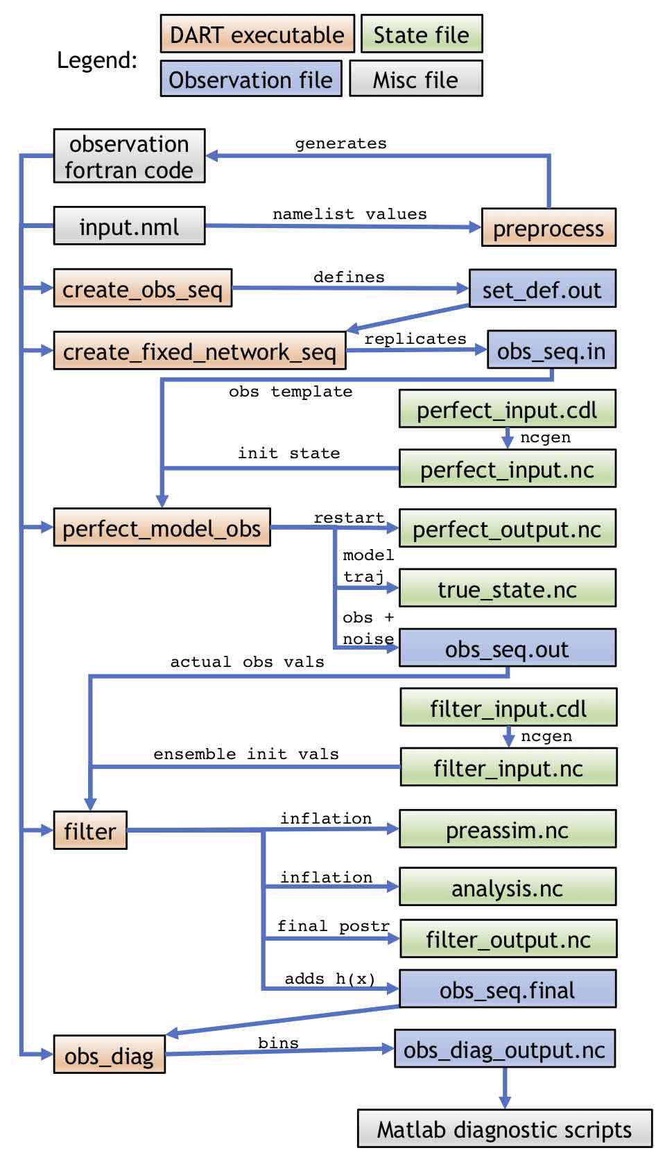
As shown, the program preprocess takes the input.nml namelist file and generates Fortran code for the observations. This code, along with the namelist, is used by all subsequent programs. create_obs_seq is used to define a set of observations in set_def.out, which can be replicated through the program create_fixed_network_seq to create a obs_seq.in file. There are two inputs to perfect_model_obs: the obs_seq.in file and perfect_input.nc (which here is generated by perfect_input.cdl via ncgen). obs_seq.in provides perfect_model_obs with the observation template (i.e. the location and type of observations), while perfect_input.nc provides the initial state that will be used to advance the model. On output, the “perfect” model state at the final time, which can be used as a restart for running this procedure again, will be written to perfect_output.nc (i.e. perfect_output.nc could be renamed to perfect_input.nc to extend the OSSE), while the entire state trajectory will be stored in true_state.nc. The noisy synthetic observations and noise-free truth (for verification only) will be stored in obs_seq.out. The observation values of obs_seq.out will be input to filter along with the filter_input.nc (generated by filter_input.cdl via ncgen), which contains the initial state for all the ensemble members. The output of filter is preassim.nc, which contains the prior state for all the ensemble members just before applying DA (so including prior inflation if it is being used); analysis.nc, which contains the posterior state for all the ensemble members after assimilation (and including inflation if it is being used); filter_output.nc, which is the final posterior that could be used to restart the OSSE process; and obs_seq.final, which adds the forward-calculated expected values h(x) for each observation. The obs_seq.final file can be analyzed and binned by the obs_diag program, producing the file obs_diag_output.nc which can be used for diagnostics.

Complex model workflow with an OSE

The second workflow is for a complex model with all ensemble members stored in separate files running an OSE. In this case, DART will only operate on one model output at a time. External programs will advance the model states, generate the observations, and call DART again. Details of DART’s internal programs, which are mentioned below, can be found in Programs included in DART. The following diagram in shows the high-level DART flow in this case:

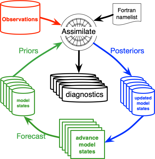
Within a single time step, DART will use the filter program to run the “Assimilate” portion of the above diagram and/or the “diagnostics” as follows:

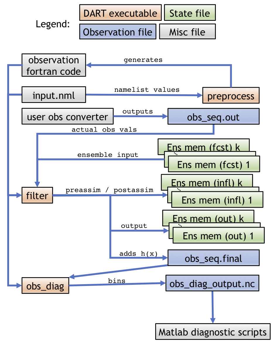
The single time-step workflow for an OSE experiment within a single step is slightly simpler than the OSSE equivalent as DART handles less of the process. Like the OSSE case, the namelist and preprocessed observation source files are input to all other DART programs. In the OSE case, however, the user must provide an obs converter that will output a obs_seq.out file. There are many DART utilities to make this process easier, but for the OSE case the obs_seq.out file is ultimately the user’s responsibility (to avoid duplicating effort, see the list of existing observation types in Important capabilities of DART). Here, the option to run with one file for each ensemble member is demonstrated. There are k ensemble members used as input to filter, which also outputs k members for the prior and posterior. The obs_seq.final and obs_diag_output.nc are used in the same way as in the OSSE case. The names of the input files and output files can be controlled by the user through the filter_input_list.txt and filter_output_list.txt files, which can contain the user-specified list of the ensemble input or output files, respectively.

Another view of the stages of filter is shown in the following diagram:

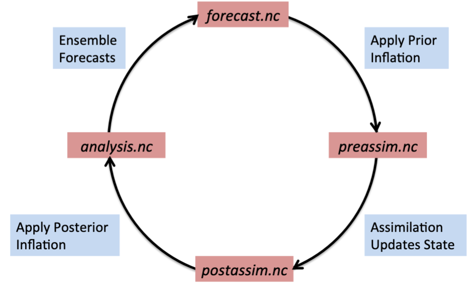
As shown here, an ensemble forecast is stored in forecast.nc , to which prior inflation can be applied and stored in preassim.nc. Once assimilation is applied, the output can be stored in postassim.nc, and finally if posterior inflation is applied, the final analysis can be written in analysis.nc . The model forecast will start from the analysis to advance the model in order to start the cycle over again.

Note

The “forecast” will be the same as the “preassim” if prior inflation is not used, and the “postassim” will be the same as the “analysis” if posterior inflation is not used. The stages_to_write variable in the “&filter_nml” section of the input.nml namelist controls which stages are output to file. For a multi-file case, the potential stages_to_write are “input, forecast, preassim, postassim, analysis, output” while for a single file the same stages are available with the exception of “input.”

Note

In the above cycling diagram, there will actually be one file per member, which is not shown here in order to simplify the process.

Important

The decision to store ensemble members as separate files and whether to run an OSSE or OSE are independent. An OSSE can be run with multiple files and an OSE can be run with all ensemble members stored in a single file.